Get Valid Answers To These Thought-Provoking Questions On Economists Production Theories

This chapter provides a general overview, giving definitions of such concepts as capital, economies of scale, diminishing returns, and different classifications of costs. Production functions and the mathematical expression of production relationships are explained. We also save you the headache of handling a delayed exam by helping you with it. Hire us to take your economics exam. Our executive microeconomics exam helpers can give you the dream grade you've always desired.

The chapter concludes with an example of how models f purchasing decisions can be simple and rewarding for the firm. Chapter 15 deals with the two best-known models of production decisions, the marginalist, and linear programming models, comparing them in theory and practice. Chapter 16 introduces some terminology and uses another linear model, input-output analysis.

Question:

What is Production?

Solution:

Economists have commonly divided microeconomics into three areas of study:

Demand theory: what is to be produced?

Production theory: how is it produced?

Distribution theory: who is to get what is produced?

This production, for managerial economists, deals with how, meaning by what combination of inputs. Things are produced. Typically the models deal with general categories like capital and Labor. Still, they apply equally to specific inputs like a man- fours of lathe operators and numbers of lathes, or gas station attendants and pumps. However, it is important to be clear on the capital defined in our model. In the short run, it usually is quite specific, several machines of a particular kind, for example; in the long run, it means the amount of money invested, which it is assumed could be spent on several different kinds of capital equipment depending on what was most profitable. It is usually obvious from the context whether the term capital' is used to represent specific machines or for the value of an unspecified mix of equipment.

It is also important to note that production is not just concerned with manufacturing. We say an activity is a product if it involves 'an expected value addition. So changing iron into steel is production because we expect the steel to be worth more than the iron and the cost of the other inputs. However, transporting goods, as is storage, is also productive when it raises their value. Thus production theory and the production decision are concerned with services, and the public sector, not just with manufacturing.

Question:

What does the economist Production Decision entail?

Solution:

To be more specific, we can see that a production decision by a firm involves, as Baumol (1977) points out, four related decisions:

The input budget.
How much of each input to purchase.
Allocation of inputs to different outputs.
How much of each output to produce.

We usually simplify the problem by assuming that we are dealing with a firm that only makes one product to clarify the principles. This enables us to eliminate decisions (3) and (4). If we also assume that the price-output decision has been taken where we have a fixed input budget. This is not unrealistic because although production costs and prices are interdependent, firms often organize production by giving production departments output targets and budgets for inputs on targeted sales. Thus many production managers are faced with just the kind of problem that the models deal with- how to produce a given output as cheaply as possible or as much as possible given a limited budget.

What information about production conditions will we need to incorporate into a model to make rational production decisions? We start by looking at how costs fall into certain patterns.

Question:

How Do Production Costs Behave?

Solution:

For a long time, economists could not decide what effect increasing output had on costs per unit. In some situations, costs appeared to rise and in others to fall. Rising costs appeared to occur when there were shortages of inputs and lower costs when new technology could be used. The explanation lay in making a distinction between the long run and the short run.

Economists commonly use four time periods whose actual lengths vary with the product concerned:

the market period when output cannot be changed, and the given stock has to be cleared from the market by lower prices or stored.
In the short run, when at least one input, usually the capital, cannot be varied.
the long run, when the inputs can all be varied.
In the very long run, when available technologies change.

In production decisions, we are concerned with the middle two periods.

The short-run

In the short run, we assume that at least one input cannot be varied but that the other, or others, can. This means we have some costs that vary with output (variable costs) and some that remain the same as output changes (fixed costs). These correspond roughly with terms used in accounting variable costs are approximately equal to Gret costs, and fixed costs are approximately eq indirect costs or overheads. Variable costs are labour and material costs; fixed costs include capital costs such as depreciation, interest payments, rent, tan management salaries, etc.

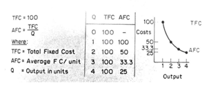
How can we expect these costs to behave a vary output in the short run? With fixed costs, the answer is purely arithmetical, as shown in Fig 14.1.

Diminishing returns

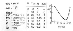
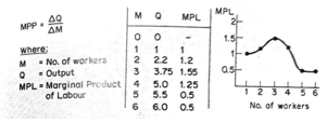
If we examine variable costs, there is no immediately obvious way they should vary with output. Conveniently we do have a great deal of evidence because, of course, firms usually operate in t situation: What we find is that in the simplest, if we consider only one factor, say Labor, a varying, its output will first rise and then fall. An example is given in Figure 14.2. The significance column is omitted from the table a marginal product of Labor, defined as the addition to output resulting from adding a worker to the labour force. In our example, we could construct Figure 14.3: M and Q are taken from Figure 14.2, and MPL is then calculated. The common way of describing the behaviour of MPL is to say that it exhibits diminishing returns, i.e. 1, the market period when output cannot be returned from Labor eventually falls. At first, we get workers (MPL rises from 1 to 1.2 to 1.55), but the MPL falls after this. The explanation appeals m commonsense; there is some normal relationship 3. In the long run, when the inputs can all be varied of capital and Labor for the particular fixed facto the very long run when available technologies in use by this firm. Below this 'optimum combination (three workers in this case), the MPL re as workers are added; beyond this ', optimum' workers will add nothing to output and after point will reduce it!

It is important to note that this property (diminishing returns) is not confined to Labor and is not a result of economic forces. It is a property of the particular kind of technology being used. Note the Labor that becomes less productive, that there is a limit to the productivity of the field factors. To take a simple example: 1 train crew c drive a locomotive for, say, 8 hours a day, hauling a given size of train: 2 crews can drive it to, say, for 16 hours, perhaps saving some light running, but three crews are unlikely to be able to drive it 24 hours a day- it has to be overhauled and repaired some time! Thus the third crew is unlikely to add as many revenue miles as the second. A fourth crew is unlikely to add as much as the third. The obvious limitation on output is the locomotive itself, and that is what the short run is all about.

Of course, the short-run analysis also applies to any situation in which factors are fixed. Thus it has historically been applied to agriculture (land is fixed in supply) or to countries (that have limited- supplies of raw materials). Finally, to spaceship earth with its finite resources. In each case, we can say that more variable factors (people or capital) will not forever send output up in proportion to the increase in variable factors. Diminishing returns are the spectre behind population and economic growth.

The long run

In the long run, we can change the amount of all the inputs used in production. This means we can choose the optimum combination of capital and labour from the known production methods. This raises three related problems with the definition of capital. How is an optimum combination chosen? And what do we mean by changing the scale of operations.

We did not have to define or measure capital in the short run because it was fixed and, therefore, not a matter of decision. However, we can now change capital, so we must know what we are discussing. Are we just interested in fixed capital such as machinery, plant, and buildings, or are we also interested in circulating capital tied up in stocks? Are accounts receivable, etc.?

The answer varies according to the purpose of our decision or, more correctly, the relevant constraints. If there are limits on the amount of capital we can use (because a firm does not wish to increase its debit unduly or a country cannot borrow from abroad), we must include working capital. If this is not the case, then we are mainly interested in the relationship between men and machines (fixed capital).

The second problem- choosing the right capital and labour combination – is easier. We shall not be looking at the most efficient way to produce and deciding the cheapest based on wage and interest rates. We shall use technical information to find out wh given capital and labour combinations produce and then decide, based on w interest rates, the cheapest way to produce a given output. This is explained more fully in Chapter 15.

Changes in the scale of output are difficult to define. Not all changes in output change in scale. The definition follows the definition of the short and long n the long run; we can change all factors, so the definition of changes in scale is when all factors dang equally. A doubling of scale world be inputs doubled in practice, we often use simplified models in which we only vary capital and laborious step and look at the net effect on output s called looking at value-added and allows the production process to become more efficient of materials, rather than expecting material increase along with capital and Labor use.

Question:

Explain factors affecting Economies of scale and how it affects fixed and variable costs

Solution:

In the same way, as we measured returns to various factors, we measured returns to changes in scale (returns to scale). The measure relates the change in output to the change in impen. For example, if output rises 100% when we increase capital and Labor by 100%, we say there are constant returns to scale. A less than 100% inc in output would have been called decreasing turns, and a more than 100% output mo increasing returns or economies of scale if there are economies of scale. Firms will tend to grow, and if not, they can choose to remain small; an enormous amount of evidence has been gathered about economies of scale, some of which is referred to in the further reading at the end of the chapter.

Fig. 14.1 How Fixed cost Vary with Output

Fig. 14.2 How Variable cost vary with Output

Fig. 14.3 calculating the marginal Product of Labor

Question:

What is a Production Function?

Solution:

Expressing the relationship between input and output in mathematical terms is called a production function. They differ in both their origin and their nature.

One important function for production has been the attempt to find a function that would reproduce such phenomena as diminishing returns of economies of scale. We call these 'theoretical functions because they have the theory first. They can be for either a firm or an industry (sometimes termed Marshallian functions after Alfred Marshall) or the economy as a whole (Walrasian after Leon Walras).

Another possible origin is in empirical investigations, seeking to find relationships between inputs and output from studying masses of data. This tends to run up against the statistical and practical problems mentioned in Chapter 13.

Perhaps the most obvious source of production functions has proved somewhat disappointing, the study of engineering data. The one area where it has proved useful is in establishing whether economies of scale exist in various industries.

Question:

State and explain the Marginalist and linear functions

Solution:

Production functions can almost all be divided up into those which are marginalist and those which are linear. Chapter 15 deals with the two approaches' main strengths and weaknesses and gives insight into their development. The next section shows how a function might be developed from known data and then used for production costs (purchasing costs in this case).

The Stockholding Model

A problem faced by all firms is the right level of stocks of finished goods to hold. With perishable (ii) w products, it seems obvious that there is an upper limit to sensible stockholding, the amount that could be sold when it takes the product to decay. Other products could be kept for a year before they became out-of-date, so they lost their value. Can we elucidate any general principles?

The first insight we can gain is that this is a typical economic problem; higher stocks mean es likelihood of being out-of-stock but costing more to store. If we remove uncertainty about demand and thus turn the problem into one of certainty, do we still have the incentive to hold large stocks? The answer is yes because if we order every week, the os will rise, both orderings costs themselves and, probably, transport costs. Ordering every week will mean smaller stockholding costs than large ordering costs; ordering once a year will mean small but large stockholding costs. We can build a cost model as in Figure 14.1. As we know from previous experience, there are two main ways of handling problems of this kind once we have a model. Simulation and use of mathematical properties ('analytical methods). Let us see how they work in this case, and see which is best.

Simulating different stock levels

We can assume that the firm will know with certainty its various costs and the annual level of sales. It is then just a matter of substituting different values of D into the equation from Table 14.1

Table 14.1 Building a stock holding cost model

(i) Q/D = Number of orders/year where	D = delivery size Q = Annual Sales W = Storage cost per unit stored
(ii) D/2 = average stockholding	a = fixed order cost b = per unit order cost
(iii) W x D/2 = Total Storage Cost
(iv) A + b x D = cost per order
(v) Total Cost = Total Storage Cost +Total Ordering Cost = WD/2 TC=WD/2	+ (i) x (v) + Q/D x [a + bD] +aQ/D + bDQ/D +aQ/D + bQ

Normally w, Q, a, and b will be known, so varying D varies TC

Table14.2 Calculation for stockholding simulation

Where:	D	TC=WD/2 +aQ/D + bQ = TC
	100	100/2+1000+2000 = 3050
W=1/Unit	200	200/2+500+2000 = 2600
a = 100	300	300/2+333+2000 = 2483
b= 2/Unit	400	300/2+333+2000 = 2483
Q= 1000	500	500/2+200+2000 = 2450
	600	600/2+167+2000 = 2467
	700	700/2+140+2000 = 2490

Table 14.3 Analytical method of minimizing stock costs

The formula is TC=WD/2 + aQ/D + b
It is easier to differentiate as TC = WD/2 + aQD-1 + bQ
Differentiating dTC/dD=W/2- aQD-2 =(0 when TC is minimized)
Thus at minimum, TC w/2 = aQD-2
As D -2 = 1/D2 then W/2 = aQ/D2
Multiplying gives WD2 = 2aQ
Dividing gives D2 = 2aQ/w
Taking the square roots D= 2aQ/W

When TC is minimized

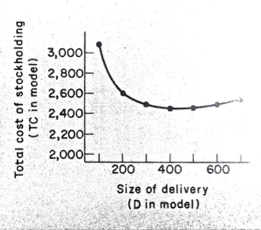
Produce the calculations in Table 14.2 and the graph in Figure 14.4. The graph clearly shows the value of D that will minimize the cost of holding stock to meet an annual demand of 1000.

Provide an analytical solution to the cost

Those who know some calculus will recognize that we have an expression for TC in which D is the only variable (in any particular case, a, b., Q and W will be constants above in Table 14.2). Thus we can say that TC will be minimized.

Let us explore the first condition: taking setting it = to 0.

Readers might like to check that the derivative is positive; the t has been minimized at the value for the D-found process. If we substitute the values for a,b, and a that we used in the example in Table 142 veg, a value for D of about 447. This agrees with a simulation that puts the lowest TC at a value of d between 400 and 500.

Thus both methods provide the same, but this example shows a clear advantage. T analytical method can be applied to any value a. b. W and without having to go through a simulation each time. One of the crucial judgments that managerial economists have to make is when a standard analytical formula can be applied and when a simulation model has to be created. One of the exercises explores the analytical formula further.

Chapter 15 looks at two more production functions where mathematical analysis has provided some interesting and rewarding might production decision-making.

Fig. 14.4 graph of stockholding simulation

Key Concepts - Review

Capital

Production

Production decision

Input budget

Long run/Short run

Variable/fixed (costs)

Direct/indirect (costs)

Marginal product (of Labor)

Diminishing returns (to an input)

Returns to scale

Economics of scale

Production functions

Simulation/analytical methods

Provide a Case Study on This Report

You work for an electricity meter manufacturer which operates on a government trading estate on the Welsh border. All the meters are brought in from Japan, recalibrated by skilled workers, and then sold to the Midlands Electricity Board, your sole customer. The firm employs nine people and has a turnover of 72,000 meters yearly for gross revenue of 120,000. The cost breakdown is as follows:

Materials (meters)	144,000
Wages and Salaries	70,000
Factory (rent, rates, heating, and lighting)	40,000
Profit	26,000
	$280,000

You have been concerned over the space taken up by stocks for some time. The finished goods are no problem; they are sent off every Thursday to Birmingham, and the lading bay w store a week's output. However, the Japanese meters come in at 18.000 at a time every three months, and half the factory space is taken up storing them. As the trading estate company only charges you for the space used, you are eager to find ways of reducing thin storage space.

The original reason for only buying every Three months was the cheaper price of a large order. You have learned that the Japanese quantity counts are based on a fused charge of $1.00 and $1.90 per meter. Your 18.000 meters cost $2 each, but if you bought every month, the 6000 meters would cost you $2.60 each.

However, a fresh complication has arisen: your boss has got an order for 1000 meters a week from the Yorkshire Electricity Board. The extra 13.000 meters needed each quarter would mean even more storage space would be needed. The trading estate has space available, and you work out t would cost about the same per square foot as your present space.

The boss wants to know whether to rent more space and whether to change the size, frequency of orders, or both. You remember seeing how the problem can be solved in a managerial economic book but are suspicious of the magic formula. You decide to work out for yourself the best size of the order, doing it in two stages, first the best order size for the present output and then the best order size, including the Yorkshire contract.