3 Questions with Answers To Help You Ace Your Next Expenditure System Midterm Exam

Are you stressed about your upcoming expenditure system midterm exam? If you are struggling with mastering the various components of national expenditure, you’ll find this blog useful. We have solved 5 questions that covers the core concepts of the expenditure systems and processes. You can use these questions and answers to improve your knowledge of national expenditure and polish your skills.

Explain the expenditure system using simple linear relationships

This is the most familiar of all macro models. It consists of an accounting identity and a number of equations determining various components of national expenditure. For the most part, simple linear relationships will be presumed.

Y = C + I + G + X – P (1.1)

National income, Y, is identically equal to consumption, C, plus investment, I, plus government expenditure, G. plus exports, X, minus imports, and P.

C = α + β ( Y – T ) (1.2)

Consumption expenditure, C, depends upon disposable income (national income, Y, minus taxes, T).

P = dY (1.3)

Imports, P, are proportional to national income, Y.

X = X0 (1.4)

Exports, X, are exogenously determined.

G = G0 (1.5)

Government expenditure, G, is exogenously determined.

I = I0 (1.6)

Investment, I, is exogenously determined.

If tax revenue is also assumed to be fixed in size, the model is 'solved' by substituting equations (1.2) - (1.6) into (1.1), to yield:

Y = α + I0 + G0 + X0 – βT (1.7)

(1 – β + d)

This is the familiar 'multiplier' equation. The multiplier tells us how much national income changes in response to changes in exogenous expenditures. Its value depends upon the size of 'leakages' from the circular flow of income; notably, in this case, the marginal propensity to save, 1- β, and the marginal (and average) propensity to import, d.

All the action in this model comes from changes in exogenous expenditures. It is presumed that there are unemployed resources so the output is entirely demand-determined. Supply factors are passive and do not enter into the determination of national income. Thus the chain of causation in this model leads from exogenous expenditures through the multiplier to national income.

This simple framework is, however, sufficient to explain the essence of the so-called Keynesian revolution. National income could settle at an 'equilibrium' in the presence of unemployed resources. This would happen if exogenous expenditures were insufficient to generate the full employment level of output. The simple solution is that government expenditure should be used, in conjunction with taxes, to stimulate the economy in times of depression and 'deflate' the economy when it is 'overheated'. This, in a nutshell, is the intellectual basis of countercyclical budgetary policy.

The model I is encaptured diagrammatically in Figure 1.1. The 45° line represents the accounting identity or aggregate supply since it represents points where domestic expenditure and output are equal.

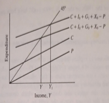
Figure 1.1 The expenditure system.

The C and P lines represent the consumption and import functions respectively. Aggregate domestic demand is given by C+10 + G0 + X0 - P. This determines an equilibrium level of national income (or output), Y. An increase in income and, therefore, of employment can be achieved by increasing government expenditure, G, to G₁. Aggregate demand thereby rises to C+10 + G1 + X0 - P and income rises to Y1 policy (that is, changes in G and T) can thus be used to regulate the level of activity in the economy.

This is the first model learned by anyone who studies macroeconomics; it is, therefore, unnecessary to dwell upon it. However, a number of points should be made which will be referred to later. The first is that all the variables in the model are in 'real' terms, i.e. they are deflated by an appropriate price index. Thus inflation has no effect since it does not shift a relationship relative to another. It is common to talk of the existence of an 'inflationary gap' where aggregate expenditure exceeds aggregate output at full employment, but inflation would do nothing in this model to resolve the such inconsistency.

Second, the model has nothing to say about the supply side of the economy. It is, in fact, presumed that resources are underemployed so it is sufficient to look at aggregate expenditure in order to explain the determination of national output. National output is demand-determined. Obviously, this has some relevance to deep depressions, but it is of questionable value in situations close to full employment. If expenditure exceeds output at 'full employment' the model becomes indeterminate. Finally, it is clear that if the workings of this economy are to be accurately predicted then the major intellectual effort has to go into the correct specification of the various expenditure functions, the consumption function being the most 'important' of these in terms of the proportion of total expenditure involved. It is a matter of some controversy whether the unemployment of the 1980s or the early 1990s could have been cured by Keynesian-style reflation.

Explain the essence of the Keynesian revolution using the money-augmented expenditure system, IS-LM

The model I was sufficient to explain the essence of the Keynesian revolution, but it was not the model of Keynes' (1936) General Theory of Employment, Interest and Money. One interpretation of this offered by Hicks (1937) included a stylised monetary sector. The monetary sector has two assets, money and bonds, the supply and demand which determine 'the' interest rate since the interest rate is the yield on bonds. Interest rate: changes affect real expenditures through investment behaviour, which is presumed to be interest-sensitive. A reverse link from the expenditure sector to money arises because the demand for money for transaction purposes increases with the level of income. Thus equation (1.6) now becomes:

I = δ – εr (1.8)

Investment is inversely related to the interest rate.

and in addition, we have equations for the demand for and supply of money.

Md = ΦY – ηr ; (1.9)

Money demand increases with income and falls with the interest rate.

Ms = M0 (1.10)

The money supply is exogenously given.

The interest rate affects the demand for money because it is the opportunity cost of holding money. (Keynes' speculative demand depends- ed on inelastic expectations but the model works in the same way.) There is no need to specify bond market equations because any financial wealth not held in money must be held in bonds. So the demand for bonds is just the inverse of the demand for money. This assumption causes difficulty if we want to analyse changes in bond sales. It then becomes necessary to incorporate a wealth constraint explicitly.

The money market can be characterised as in Figure 1.2 where the money demand line is drawn for a given Y. The M, line traces the relation between r and money demand, or speculative demand. At higher levels of Y the M, line shifts up because more money is demanded for transaction purposes. Thus for a given money supply higher levels of Y will be associated with higher levels of the interest rate, r. In the expenditure sector, higher interest rates produce lower levels of income Y. This is because the increased interest rate reduces investment, which through the multiplier process reduces income.

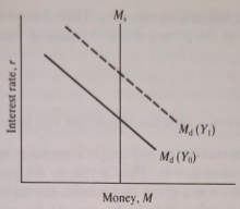
Figure 1.2 The money market

Thus, we cannot solve the monetary sector or the expenditure sector separately since the outcome of each affects the other. The procedure adopted is to trace out two loci of combinations of interest rates and income which are associated with equilibrium in each sector separately. Where these two lines cross, the values of Y and r so determined will be equilibrium values for the model as a whole. In Figure 1.3 the line LM is made up of combinations of Y and r that are associated with equilibrium in the money market (i.e. demand and supply of money are equal) and the line IS is made up of combinations of Y and r associated with equilibrium in the expenditure sector (i.e. injections equal withdrawals). The IS and LM

curves are derived algebraically in the appendix to this chapter. This model still has variables determined in real terms. The money price level does not change, so changes in Y are changes in real output. It is, however, possible to allow changes in the price level but only at the expense of fixing real income Y, say at full employment, Yo- Then Y is no longer a variable and p is introduced in the money demand equation which now becomes:

Md /p = - ηr (1.11)

Real money demand depends upon the interest rate with income fixed.

The change arises because, whereas the money supply is nominal, money is demanded its real purchasing power. Thus a rise in the price level reduces the real money supply. For a given real income the interest rate equating money demand and supply will be higher for a higher price level and for a given nominal money supply. To see this, relabel the horizontal axis in Figure 1.2 M/p and shift the M, the line to the left. For a given Ms, Ms/p gets smaller as p rises.

The relevance of this modification to the model will appear below but it does illustrate one case of interest. If, when full-employment real output is fixed, the money supply is increased, the net result will be an increase in the price level proportional to the increase in M. This is the classical quantity theory result and it arises because all the real variables in the system are assumed to be fixed. As a result, there can be only one real money stock, in equilibrium. An increase in the nominal money stock will be eroded by a rise in prices until the real money stock of the initial situation has been restored. However, this tells us nothing about the rate of inflation since we have a comparative static model, not a dynamic one. We know that a once-and-for-all rise in the money supply will produce a once-and-for-all rise in the price level, but we cannot say what the time path of this adjustment will be.

Returning to the model where real income is variable and prices are fixed, it is worth noting how monetary factors influence real behaviour. A change in the money supply does not directly influence expenditures. Rather, it leads first of all to a readjustment of portfolios. An excess supply of money is an excess demand for bonds. This leads to a rise in the price of bonds, which is equivalent to a fall in the rate of interest since the bonds are perpetuities. Only in so far as expenditures (of any kind) are interest-sensitive will there then be any real changes in response to the initial money supply increase. An important point is involved here since researchers working in the 1960s on UK data found it difficult to pick up interest effects in the aggregate investment relationship (save for housing) and thus concluded that money is of little importance. However, more recent research has established clear links between interest rates and not a fixed investment and stock building, but also consumption. Moreover, it is quite possible that the link from money to expenditure is more direct. An excess money supply is spent, not just on bonds, but also on goods.

If it were the case that an excess supply of money was spent directly on goods this would mean that evidence on the interest sensitivity of investment would not be important for judging the impact of money on the economy. Instead, we should expect to find terms in excess money balances appearing in expenditure equations such as the consumption function. It is difficult to incorporate asset stocks in expenditure functions short of specifying a full intertemporal optimisation model in which the time paths of expenditures and assets are simultaneously chosen. The whole attraction of the IS-LM set-up is exactly that the separability of expenditures and asset choices provides for welcome simplicity.

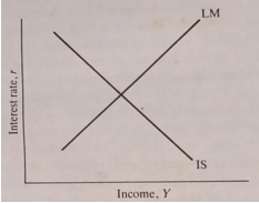
Figure 1.3 Equilibrium aggregate demand.

How can the concept of demand and supply be used to explain aggregate expenditures?

The third commonly used model adds a supply side to the economy. Models I and II are essentially ways of explaining aggregate expenditures. The addition is now made of a productive sector within which the level of employment is determined as well as the level of real output. It is effectively assumed that the capital stock is fixed. There is, therefore, a production function relating output to the input of the variable factor (labour). Labour is hired up to the point where the value of the marginal product of labour is equal to the wage rate, and the supply of labour is also assumed to depend upon the wage rate.

Y = f (K, L) (1.12)

Output is a function of capital and labour.

Ld = θ (w) (1.13)

Labour demand depends upon the wage rate.

Ls = μ(w) (1.14)

Labour supply depends upon the wage rate.

The equilibrium in this sector can be illustrated with regard to labour demand and supply alone (see Figure 1.4). Two important points need to be stressed. First, increases in employment will be uniquely associated with increases in real national output and vice versa. This is because we have a given production function (1.12) in which labour is the only variable input. Second, we need to consider whether the labour demand and supply curves depend upon the money wage rate or upon the real wage rate (i.e. the money wage rate deflated by the price index of output).

A moment's thought should make it clear that firms should only be interested in the real wage rate. If the price of output and the money wage rate increased together then the levels of real output and employment at which the money wage is equal to the value of the marginal product of labour will be unchanged. Thus it is reasonable to presume that the demand for labour depends upon the real wage. So far as the supply of labour is concerned, it would be rational if this depended upon the real wage since leisure is effectively forfeited for the goods that wages will buy. However, it is sometimes assumed that workers do not fully appreciate or anticipate the extent to which money wage increases are offset by price increases Accordingly, it is worth pursuing two alternative assumptions with regard to labour supply. The first is that labour supply depends upon the real wage, and the second is that it depends upon the money wage or, equivalently, that workers offer labour based upon the expected price level and expectations lag behind the reality.

If both labour demand and supply depend upon the real wage then output and employment will be determined independently of nominal prices and wages. An increase in the price of output, accompanied by a rise in money wages, would have no real effect since the real wage would not change. However, if labour supply depends upon the money wage, an increase in money wages accompanied by a proportionate rise in prices would increase labour supply. In this case, both prices and real output would rise. Workers would, in effect, be suffering from the illusion that their real wages had risen and would be acting as if labour supply depending upon the money wage.

It is now possible to derive what can be called aggregate demand and supply curves with both price level and real income as endogenous variables. The aggregate supply curve is implicit in what has just been discussed. In the case in which labour supply depends upon the real wage, varying the price of output will leave the real value of output unchanged. Nothing concrete in the productive sector changes because all nominal values (i.c. prices expressed in terms of the numeraire, money) move together, and there is no change in relative prices. Here the aggregate supply curve, Figure 1.5, is vertical since the output is fixed independently of prices.

The situation is very different when labour supply is an increasing function of money wages, or workers act on price expectations which are incorrect. any rise in money wages is perceived as an increase in real wages so more labour is offered. If prices rise but money wages rise less quickly, there will be an increase in labour supply (money wage has risen) and at the same time, an increase in the quantity of labour demanded (real wage has fallen). Thus there will be an increase in employment and real output. In short, on the assumption that there is some money illusion on the labour supply side, as prices rise there will be an increase in the supply of output. The aggregate supply curve will be positively sloped. This version we call Model IIIA. Let the vertical aggregate supply be Model IIIB. The latter can be thought of as the long-run situation when workers come to anticipate the price level correctly. The former can be thought of as the short-run case when price rises are not fully anticipated. It is this distinction between anticipated and unanticipated changes in aggregate demand that is central to New Classical economics (see Chapter 4); for a text which develops this approach, see Parkin and Bade, 1982. Their conclusion that only unanticipated aggregate demand policy has real effects depends entirely on this distinction between Models IIIA and IIIB.

Derivation of the aggregate demand curve is entirely from the money-augmented expenditure system Model II (see the appendix to this chapter). It was noted earlier that Model II could be used to determine either real income or the price level but not both. However, it should now be noted that, for given values of all the exogenous variables (especially the nominal money supply), a higher price level will be associated with a lower level of real income. This is not because a higher price reduces the quantity demanded as in a single market demand situation. Rather, it is because, for a given nominal supply, a higher price level reduces the real money supply. As a result, the LM curve shifts to the left, the interest rate rises and real expenditures fall. Real income therefore falls. Thus, the aggregate demand curve, drawn between the price level and real income, is negatively sloped, Figure 1.5. Higher price levels are associated with lower levels of real income when Model 11 is considered alone.

A simple example will serve to illustrate how the full model works. Anything in Model II would have shifted the IS curve to the right or the LM curve to the right will shift the aggregate demand curve to the right, i.e. an increase in exogenous expenditures or an increase in the money supply. Only an increase in the supply of factors of production or a technical change in the production will shift the aggregate supply curve to the right. Consider then an increase in exogenous investment in Figure 1.6. The upper half of the diagram shows the IS and LM curves, and the lower half shows the aggregate demand and supply curves.

The initial effect of an increase in investment is to shift the IS curve to the right, IS0 to IS1. In Model I, income would increase as a result of the simple multiplier to Y3 In Model II the increase in income is less than this because the increase in income raises transactions demand for money and, therefore, bids up the interest rate. This increase in the interest rate reduces endogenous investment, which in turn reduces income. Thus in Model II income increases to Y2 (Y₂ < Y3).

Y2 would only be the outcome in Model III if the aggregate supply curve were horizontal, i.e. if all the output demanded were forthcoming at a fixed. price level. It has been seen above that this is not likely. For the money illusion or short-run case there will be some increase in both the price level and real output. The aggregate supply curve, in this case, is Sa National income will rise to Y1. This is smaller again than Y2 The reason for this is that the increase in the price level has reduced the real money supply so the LM curve has shifted to LM1 thereby increasing the interest rate and reducing endogenous expenditures still further.

Where the aggregate supply curve is vertical, SB (i.e. the long-run case where there is no money illusion on the labour supply side), there is no increase in real national income or output. It stays at Y0. In this case, the initial increase in exogenous expenditure leads only to a rise in the price level, from P0 to P₁. As a result the LM curve shifts to LM2 such that its intersection with IS, is at exactly the original level of real income.

Each new model in this chapter represents an extension of the previous one. The above example shows clearly how the predictions change as we move from one model to another. For a given shift in exogenous variables, Model I predicts the greatest effect on real income since real variables are the only ones to adjust. Model II reduces the real effects by adding interest rate feedback. Model IIIA reduces the real effects still further by adding price-level feedback. Finally, in Model IIIB, real effects are entirely eliminated and the adjustment is entirely in terms of the price level, interest rates and other nominal values.

The term 'Keynesian' in macroeconomics is normally associated with Models I and II (although there is an amorphous 'New Keynesian' school which we consider in Chapter 5). Keynesians presume that increases in aggregate demand will produce significant increases in aggregate supply (except at full employment). Monetarists are associated with the position that, in the long run, increases in nominal aggregate demand will mainly be reflected in prices, with output tending to some 'natural' rate. The main difference between Monetarists and New Classicists is with respect to short-run dynamics. Monetarists believe that prices are sticky so there are 'long and variable lags' in the adjustment process. A Monetarist would expect there to be temporary output changes in response to aggregate demand increases until prices have adjusted. In New Classical economics the price change is immediate if the aggregate demand change is anticipated. Model IIIA would thus be the Monetarist case during the adjustment period and it would be the New Classical case for unanticipated demand shocks. Model IIIB would be the long-run case for Monetarists and New Classicists, and it would also be the short-run case for the latter when demand changes are anticipated. While New Classical economics assumes price flexibility, it is necessary to adduce other forms of stickiness in order to reconcile their models with real-world data which exhibit obvious patterns of persistence.

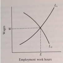
Figure 1.4 Labour market equilibrium.

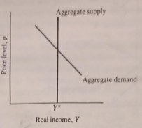
Figure 1.5 Aggregate demand and supply.

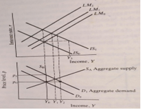
Figure 1.6 The full model.