Online Aggregate Demand Exam Tips For University Students
Analyze the growth of aggregate demand using the Philips curves
Consider the course of inflation and unemployment that would occur if the economy were initially at the NAIRU with zero inflation and zero growth of aggregate nominal demand and the growth rate of aggregate demand is raised to 10 per cent. What happens?
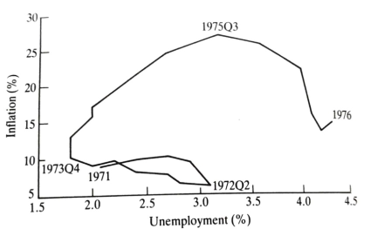
Figure 7.6 Budget Constraints
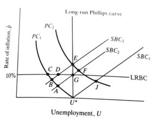
Figure 7.7 Short- and long-run Philips curve and budget constraints
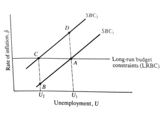
Figure 7.8 Retail price inflation and UK unemployment: 1971-76
Explain using a graph how inflation and unemployment impacted the economics of 1978-82
As Figure 7.9 graphically demonstrates, the economy did not home in on 4 per cent unemployment. Rather, unemployment accelerated dramatically from early 1980 to reach a level of nearly 12 per cent in early 1983. It is true that inflation had also come down to about 5 per cent by early 1983, but on the basis of previous patterns this should have been possible at very much higher levels of employment. The rise in inflation from 1978 to 1980 may be explicable in terms of a number of temporary factors such as the 1979 oil price rise and the increase in VAT resulting from the June 1979 Budget. The real problem, however, is to explain the massive rise in unemployment. Earlier in this chapter we set out a bargaining model of the labor market which is now more or less the conventional view. It offers a synthesis of demand and supply-side effects; we can analyze changes in unemployment in terms of either demand or supply-side forces. For example, if the demand for output and therefore labor collapses and if wages do not immediately respond to the changed conditions, then unemployment will rise. Alternatively, if (say) there were an increase in the mismatch between the unemployed and vacancies, then the natural, NAIRU and subsequently actual rates would rise. Which factors matter is an empirical question? The most comprehensive (and comprehensible) account of the UK experience is given in Layard, Nickell and Jackman (1991), where the results from the Centre for Economic Performance) research into the causes of unemployment are set out LSB Centre for Labor Economics (now Broadly speaking, a given rise in unemployment can be broken down into three components: a rise in equilibrium unemployment (the NAIRUS in demand, and dynamic effects (which can be very long lived, more so the United Kingdom than in many other countries). Table 7:1 summaries their findings with respect to the first component.
The table shows that one popular explanation of the rise in unemployment can be dismissed straightaway. That is, that high unemployment benefits shifted the natural rate of unemployment so that millions of workers chose to be out of work, the utility of not working being greater than that in work. This explanation, although popular, was always preposterous. It is undoubtedly true that the level of benefits has a marginal effect on the level of measured unemployment, but it is absurd to suggest that this can explain job losses in Britain in recent years. As the table shows, the effect is absolutely minimal; but other supply-side effects do not really add up to much either. There appears to be a small effect arising from mismatch and from an improvement in the terms of trade (import prices) which drive a wedge between producer and consumer prices, but the total effect (comparing the period 1974-80 to 1980-87) is less than per cent, compared to a rise of nearly 6 per cent in the actual 10
This means we must look elsewhere for an explanation of the rise. On the unemployment rate. Supply side, Layard, Nickell and Jackman (1991) believe that their econometric results exclude two crucial variables. First, they argue that there has been an increase in the degree of skill mismatch in the 1980s which is not picked up by their indicators. As evidence, they give the ratio of firms reporting shortages of skilled to unskilled labor (from the Confederation of British Industry (CBI) survey). This ratio was 2.73 in the 1960-74 periods, but rose to 6.92 in 1981-87.
Table 7.1 A breakdown of changes in the UK NAIRU
| Percentage Points | 1967-73 to 1974-80 | 1974-80 to 1980-87 |
| 1974-80 to 1980-87 | -0.28 | -2.58 |
| mismatch | 0.55 | 1.54 |
| import prices | 1.49 | 1.27 |
| benefits | -0.29 | 0.48 |
| unions | 0.82 | 0.08 |
| tax wedge | 0.03 | -0.32 |
| Total Effect | 2.32 | 0.46 |
| Actual Rise | 1.84 | 5.91 |
The other factor is the treatment of the unemployed. They believe that compared with the 1950s and 1960s, the unemployed were treated more leniently by the social security and unemployment registration systems in the 1970s. Society was also more tolerant towards individuals who found themselves unemployed. These changes were due partly to institutional changes like the separation of unemployment benefit administration and registration for job search; the former is administered by the DSS, while the latter takes place at Department of Employment job centre. Another hard to quantify factor is the insidious effect of the growth in unemployment itself, eroding the work ethic (and also general skills)." So unemployment became less of a threatening experience, and less pressure was placed on the unemployed to search for new jobs.
Yet no-one argues that the exceptionally rapid rise in unemployment between 1979 and 1981 was mainly caused by supply-side phenomena. The culprit must be demand. This raises the question of where the impetus came from. One suggestion is that Britain suffered from a decline in world trade. There is a modicum of truth in this, but it can explain only a tiny fraction of the problem. World trade in manufactures, in fact, continued to grow in volume terms until sometime in the middle of 1981. Indeed, British exports of manufactures in volume terms were virtually constant in the four years 1977-80, and declined by only about 4 per cent in 1981 to then level off for 1982. The events of importance for employment precede this drop in exports by between one and two years.
Another explanation which has more widespread support is that the British economy suffered a massive ('Monetarist') deflation of domestic aggregate demand through cutbacks of domestic expenditures. Perhaps surprisingly, this is also hard to sustain. Table 7.2 shows the breakdown of expenditures in constant (1985) prices. The two major categories of spending -personal consumption and government current expenditure on goods and services - have a rising trend throughout the period. Investment declines but only latterly and there are a running down in the last two years of the stocks built up in the 1976-79 period.
Table 7.2 Expenditure (m 1985 prices)
| Year | Total | Consumers expenditure | Government expenditure | Investment expenditure | Change in stocks |
| 1974 | 300 057 | 178 216 | 63 598 | 54 465 | 2980 |
| 1975 | 294 668 | 177 500 | 67 147 | 53 383 | -3402 |
| 1976 | 302 547 | 178 279 | 67 977 | 54 277 | 1622 |
| 1977 | 301 583 | 177 483 | 66 855 | 53 307 | 3416 |
| 1978 | 314 247 | 187 510 | 68 400 | 54 914 | 2867 |
| 1979 | 325 813 | 195 664 | 69 776 | 56 450 | 3328 |
| 1980 | 316 602 | 195 825 | 70 872 | 53 416 | -3371 |
| 1981 | 311 634 | 196 011 | 71 086 | 48 298 | -3200 |
It could be argued that this shows that the 'transmission mechanism is through high real interest rates causing a fall in investment and a rundown of stocks. This is certainly contributory, but it is not the main event. Notice that the volume of demand in 1981 is about the same as in 1978 and yet between those two dates unemployment more than doubled. Notice also that the rundown of stocks in 1980 and 1981 was still less than the build-up in the previous four years. This suggests that we look to these earlier years consumption was rising steadily and yet domestic manufacturers were and ask why it was that stocks of unsold goods were building up. Domestic producing more than they could sell. How can these apparent inconsistencies be reconciled?
A major part of the answer turns out to be remarkably simple. It is that there was a substantial shift of domestic demand away from domestic manufactured goods towards imported manufactured goods. This is graphically illustrated by Table 7.3. There was a 66 per cent increase in the volume of imports of manufactures between 1975 and 1982, with the bulk of the rise coming before the end of 1979. Notice that manufactured imports and exports move together until after 1977 when exports level off and imports accelerate. The switch does not produce an immediate decline in production by domestic industry. Rather, they build up stocks of unsold products, as we have seen. As Figure 7.10 reveals, the production pattern changes dramatically after 1979. Between late 1979 and the end of 1980 there is a massive fall in industrial production of the order of 15 per cent. This fall is largely over by 1981, though the annual average figures look like they continue to fall (the average index for 1980 is higher than the index at the end of the year). This fall in production is clearly correlated with the period of rapidly rising unemployment and precedes it by some months Production starts to dive in late 1979 and unemployment starts to accelerate in early 1980.
Table 7.3 Imports and Exports of fuel and manufacturers (1985=100)
Imports |
Exports |
|||
|---|---|---|---|---|
Year |
Fuels |
Manufactures |
Fuels |
Manufactures |
1973 |
227.9 |
45.2 |
22.5 |
74.1 |
1974 |
21301 |
48.3 |
21.0 |
79.2 |
1975 |
173.7 |
43.5 |
19.3 |
76.8 |
1976 |
174.0 |
48.3 |
23.2 |
83.2 |
1977 |
143.7 |
52.3 |
32.1 |
88.3 |
1978 |
139.1 |
59.7 |
40.4 |
89.8 |
1979 |
137.0 |
69.1 |
58.4 |
88.5 |
1980 |
115.4 |
65.1 |
58.2 |
87.2 |
1981 |
94.3 |
68.3 |
70.2 |
84.7 |
1982 |
86.0 |
75.9 |
77.6 |
85.2 |
The speed of this adjustment presumably owes something to high interest rates, but it should be clear by now that this is not the major cause. There had been overproduction for some years. The problem was that domestic firms had, over successive years, lost their grip on the home market. There was no compensating expansion of exports. This increase of import penetration was not due to an upsurge of incompetence on the part of domestic producers. Rather, the explanation is to be found in the fact that this is the period of maximum expansion of North Sea oil production. Table 7.3 shows the steady decline of fuel imports and rise in fuel exports. This is associated with a substantial appreciation of sterling as we saw in Chapter 6. This appreciation of sterling, remarkably, had only a minor effect on the volume of manufactured exports, but it had a substantial effect on imports of manufactures. Domestic producers were squeezed out of the home market. The effect on employment lagged behind output somewhat. The reason is that producers failed to appreciate what was happening to demand; the CBI survey of output expectations shows that expectations were consistently over-optimistic throughout this episode. This also explains why firms found themselves building up stocks at such a rate. Despite the fall in stocks in 1980 and 1981, the ratio of stocks to output was higher throughout 1982 than in any period in 1977 or 1978.