Guidance for online Inflation and Unemployment Midterm Exams

Are you having trouble completing your midterm inflation and unemployment exam? Here are some practice questions to help you master the popular concepts of inflation and employment. Our top-rated test takers have answered the questions in detail, using relevant diagrams and examples to make the solution easy to understand. Remember we are at your service round the clock. Feel free to contact us if you need assistance with any exam related to inflation and employment.

Why were the economic policies formulated in the 70s dominated by the problem of inflation?

Between 1951 and 1967 the rate of inflation in the United Kingdom tee exceeded 6 per cent per annum. In 1975 it was of the order of 25 per c per annum. It should, therefore, be no surprise that economic policy of the 1970s was dominated by the problem of inflation. By mid-196 inflation had fallen to nearly 2 per cent, and although it rose subsequently it was back under 2 per cent in 1993. In contrast, unemployment drifted upwards. In 1955, it was 1.1 per cent of the labor force, but in 1974 was 2.0 per cent' (a level sufficiently high to prompt the famous U-turn of the Conservative administration led by Prime Minister Edward Heath). By 1979 it was at 4.1 per cent, prompting the Conservative opposition to coin the phrase 'Labor isn't working', which, in the light of subsequent events, was to prove highly ironic. From early 1980 unemployment accelerated dramatically, reaching about 10 per cent by early 1983. Between the beginning of 1980 and the end of 1982 about 1.7 million jobs (net) disappeared in the United Kingdom. When the upturn came, unemployment fell almost as precipitously, from 11.2 per cent a 1986 to 5.6 per cent in mid-1990, but subsequently rose again, to 11.0 cent in April 1993. It is incumbent upon economists to offer some explanations of these dramatic events which have been variously blamed upon declines in world demand, excessive unemployment benefits, Monetarist deflation, variations in house prices and many others.

In this chapter we concentrate on the period up to 1985, leaving discussion of the more recent past to the following chapter. We begin by examining the development of analytical models of the interaction inflation and unemployment.

Explain how the Philips curve is used to explain the dynamic behavior of a macro model

One of the most famous relationships in macroeconomics is the inverse relationship between inflation and unemployment identified by A. W. H. Phillips (1958) and hence known as the Phillips curve. This relationship was, however, pointed out much earlier in the United States by Irving Fisher (1973). Further important supportive work on the Phillips curve was done by Lipsey (1960).

The problem Phillips posed for himself was how to explain the dynamic behavior of a macro model such as Model II when it was close to full employment. The textbook models had real output changing only at less than full employment, whereas at full employment only prices changed. Phillips focused particularly on the labor market and proposed that as the pressure of demand, as measured by unemployment, got greater and greater, the rate of increase of wages would rise. As a zero level of unemployment was approached the rate of increase of wages would approach infinity. Phillips showed that the evidence of nearly 100 years was consistent with the existence of a stable relationship, as depicted in Figure 7.1. The theoretical underpinnings were refined by Lipsey who worked in terms of separate wage and price equations. Wages were determined by unemployment, and prices were determined by a mark-up on wages plus other costs. Followers often dropped this refinement and simply drew Figure 7.1 with inflation, p. on the vertical axis instead of w. It is now a commonplace to draw the Phillips curve as a relationship between p and U. and this practice will be continued below.

The Phillips curve was widely adopted by economists in the early 1960s as filling in a gap in the standard version of Model II. During this period it was generally accepted that inflation was mainly caused by demand factors, though even Phillips was fully aware that cost factors, especially import prices, could exert an independent influence on the price level. However, they had not often done so in the previous 100 years. Recent work on price determination (for example, Price (1991)) makes it clear that elements costs other than wages are important in the determination of prices though it is no surprise that the evidence only becomes econometrically visible after the 1970s, as before then there was very little variation in raw material and energy prices.

After devaluation in 1967 the inflationary experience was considered worse than previously, as Phillips himself would have predicted. Wage however, lagged behind prices owing to the incomes policy of 1968-69 and also presumably because people did not know what to expect in terms d price rises. The resultant 'wage explosion' in 1969 was widely interpreted a proving the possibility of wage push independent of the level of demand However, it can also be interpreted as a catch-up of expectations. Lade (1976) argues that over this period the country was merely reimporting the inflation it had previously been exporting.

Even if the data from the late 1960s could be made to fit with the Phillips curve, the data from the 1970s certainly could not. Indeed, de theoretical basis of the simple Phillips curve had been undermined independently by Phelps (1968) and Friedman (1968) long before even had made this reappraisal necessary. The Phelps Friedman approach forms the starting point for the model to be developed below.

An essential ingredient of the modified approach to the Phillips curse's the idea that workers and firms bargain over real, rather than nominal wages. Thus the Phillips curve has to be shifted up for each level of expected inflation to take account of the anticipated erosion of purchasing power over time. There is then a short-run trade-off between inflation and unemployment for each given expected rate of inflation- but the story does not stop there. Not only does the short-run Phillips curve shift over time as inflation expectations change, but the long-run position may also alter. We return to these issues in more detail below.

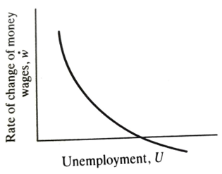
Figure 7.1 The Philips curve

Discuss the major disagreement in the causes of inflation in relation to aggregate demand and supply

The major disagreement over the causes of inflation is often characterized as being between those who think it comes from aggregate demand and those who think it comes from the supply side of the economy. Most would agree that an expansion of the money stock is necessary to sustain a price-level rise, but those who believe in cost-push usually argue that the money stock has to be expanded in the wake of inflation to avoid unemployment. Both lines of argument could be valid. The question & what actually happened in any particular episode? Let us first look at the price level and the level of output in terms of Model III. Following Gordon (1978) it is convenient to combine the two versions

Model III a simple modification of the aggregate supply curve. For the short-run case where money illusion was assumed on the part of suppliers of labor, we assume that labor supply depends upon the expected price level Demand for labor on the other hand depends upon the actual price level. In the short run, while expectations lag behind reality, the aggregate supply curve will be upward sloping but it will shift leftward if expectations are revised upwards. In long run expectations are correct so the long-run supply curve is vertical at the trend output level sometimes called the natural" output level. In other words, the long-run supply curve shifts rightwards each period because of the underlying growth of the economy. If we consider the initial position in Figure 7.2 to be at point A then it is dear that a price-level rise can be started by either a rightward shift of aggregate demand AD,, or a leftward shift of aggregate supply. A cost-induced inflation would involve a supply-side shift and the economy would move from A to C. A move to D would then follow if measures were taken to eliminate unemployment. Eventually the system would settle again at a higher price level on the long-run aggregate supply curve. A demand-induced inflation, however, would be caused by a shift of the demand curve to, say, AD, so the economy would move from A to B. Expectations would then be revised so that AS, would shift in the direction of AS, and the economy would move to a point like D. Whether D is in this case to the left or right of long-run AS does not matter- either is possible. The point is that a demand-induced inflation will move the economy through an anti-clock wise arc initially. A supply-induced inflation will move it through a clockwise arc.

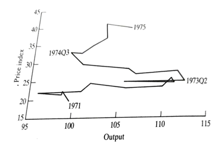
The picture in the United Kingdom in the early 1970s is extremely clear, as Figure 7.3 shows, so long as it is appropriate to start the cycle in 1971. The end of 1971 marks the beginning of a major expansion of the money supply associated with Competition and Credit Control, and March 1972 was the date of Mr Barber's famous expansionary budget. Hence a shift of demand moves the economy along a short-run supply curve, which incidentally appears to be fairly flat. After the oil shock (and a further supply-side squeeze following from a spectacularly badly timed attempt to introduce indexed wage contracts just when retail prices were unexpectedly rising steeply) there is a dramatic leftward bounce in output to the trough in late 1974. While the adverse supply shift does not go away, the effects of the Barber boom persist and the economy slides up the short-run supply curve as demand recovers.

Notice that while the movement from 1973 to 1975 must involve a shift of the supply curve, some such shift would be an essential part of the demand- induced story. The economy cannot stay at a point like B in Figure 72 because it is beyond the long-run supply curve. Price expectations will necessarily shift the supply curve leftward sooner or later. It is quite likely that the oil price rise induced the shift of supply between 1973 and 1975, but it is important to realize that after the events of 1971-73 some such shift would have occurred anyway due to the behavior of expectations.

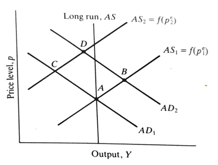
Figure 7.2 Aggregate supply and demand with price expectations

Producer prices and manufacturing output in the United Kingdom

Discuss using a diagram the expectations of the augmented Philips curve

An analogous argument can be developed in the more familiar dimensions of inflation and unemployment. It was seen above that a single stable Phillips curve is incapable of reconciling the observation of both high inflation and high unemployment. However, once it is admitted that there is a new higher Phillips curve for each higher expected rate of inflation events become easy to explain.

To see this, suppose curve PC, in Figure 7.4 is the Phillips curve for zero expected inflation. If the level of unemployment is U, this expectation will be fulfilled and nothing needs to change. However, if unemployment were U inflation would be greater than zero at p. In effect, the wage bargainers made a mistake setting wages inflation turned out to be higher than they expected (the expectation error is positive). Friedman, using a form of adaptive expectations, argued that having underestimated inflation, the nest period expectations would be revised upwards. This generates a higher Phillips curve, says PC, Again, inflation would be higher than expected and, so long as unemployment stayed at U, inflation would accelerate. So long as we remain to the left of U. inflation carries on increasing consequently, we call this the 'accelerations' hypothesis. We can think of the long run as the period within which expectations are fulfilled. As a result, the long-run Phillips curve traces out the point on each short-run curve where expectations will be fulfilled and where inflation is consequently stable. The dramatic conclusion is that the long-run Phillips curve is vertical by definition. There can be no long-run trade-off between inflation and unemployment.

Friedman referred to the unique level of unemployment at which expectations turn out to be correct as the Natural Rate of Unemployment, also known as the equilibrium rate. He made very large claims for this rate, which we now know to be unjustified:

The natural rate of unemployment is the level that would be ground out by the Walrasian system of general equilibrium equations, provided there is embedded in them the actual structural characteristics of the labor and commodity markets, including market imperfections, stochastic variability in demands and supplies, the cost of gathering information about job vacancies and labor availabilities, the cost of mobility, and so on. (Friedman, 1968, p. 8)

'Natural' carries with it the implicit connotation that it is also 'best' but the equilibrium rate, even in the absence of powerful unions, will generally be inefficient. This is not the place to rehearse the arguments, but it turns out that the natural rate may be too high or too low, as the factors pushing is away from efficiency can go either way; see Pissarides (1990) for an exhaustive discussion of the issues. Thus a preferable, less value-laden, term for the unique long-run level is the NAIRU, or Non-Accelerating Inflation Rate of Unemployment. However, the term 'Natural Rate' is still a useful one to keep. As we see below, the concept of the NAIRU can be fitted into the wage bargaining model set out in Chapter 5, and it is useful to think of the natural rate as the level of unemployment that would prevail in the absence of any union bargaining power. It is important to bear in mind that it is unlikely to remain constant over time. For instance, if unemployment benefits fell it is likely the unemployed would want to spend less time searching for work, and the natural rate would fall. This will affect the NAIRU. However, as we will see, other factors (such as trade union legislation) can also affect the NAIRU, even if the natural rate is constant.

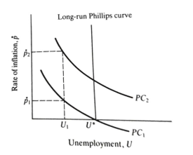
Figure 7.4 Shifting Philips Curve

Using Friedman’s version of the Philips curve, explain how the Philips curve shifts in a unionized economy like the United Kingdom

Friedman had in mind a competitive world where atomistic firms compete and individual workers search for work. What drove his version of the Phillips curve were unemployed workers mistakenly accepting high money wage offers, wrongly thinking that they were high real wages. In order to understand how the Phillips curve shifts in a unionized economy like the United Kingdom, we have to consider the bargain struck between firms and workers.

The issue of firm/union bargaining was addressed, and this section builds on that analysis. As argued in that chapter, firms and unions both have ideal targets for the real wage. The firm would like wages to be set at the minimum market rate. This sets a floor; if the wage were any lower, the firm would be unable to employ enough workers. Ceteris paribus, unions want a higher wage, but as they recognize that higher wages imply lower employment, their ideal wage takes into account the consequences for jobs, balancing higher wages with laid-off union members. We assume that firms have the 'right to manage', so we are always on the demand curve. While this is technically inefficient, as discussed in Chapter 5, the evidence is that it is the realistic assumption. This leads to Figure 7.5.

The figure assumes there is only one (representative) firm so we can work directly with unemployment. Thus L is the conventional labor demand curve, which slopes upwards when unemployment (rather than employment) is on the horizontal axis as drawn here, and L' is labor supply. Vis the union's ideal point, with associated real wage WT; F is the firm's ideal at the competitive wage W. The actual outcome is at Wo and Uo. The determinants of Wo (and therefore U) are the factors that affect the target wage, the competitive wage, and the union's relative bargaining power. The competitive wage can be thought of as being determined by the natural rate of unemployment; if this increases, effective labor supply falls and the competitive wage rises. So anything that affects the natural rate affects the competitive wage. Factors likely to increase the natural rate are the degree of mismatch or 'noise' in the labor market, like the disparity between the type of jobs available and the skills of those unemployed; the level of unemployment benefits, which affects the length of time the unemployed spend hunting for a job; and institutional factors like the social stigma attached to unemployment, or the administrative structure of the government employment services.

The union wage will similarly be affected by several factors. These include union preferences; if unions become more 'militant' it may be reflected in a push for higher wages. Other factors include the level of unemployment benefits or wages in any non-union sectors, which soften the impact of job losses on union members, and the level of aggregate unemployment itself. The higher is unemployment, the more serious is the effect of a lost job, as laid-off workers tend to spend longer between jobs.

The actual outcome will depend on the relative bargaining strength of the two parties. This will be affected by legislation, and also by the ability of one party to impose costs on the other. For example, a high level of capita intensity makes it easy for workers to impose large costs on employers i the event of a strike, as although there are no wage costs during a strike capital and other fixed costs are still incurred. Strikes might also be more effective when demand for the product is buoyant, as lost profits a Finally, note that a contraction in demand (a rightward shift in Lin Figure 7.5) will tend to lower the bargained real wage, as the competitive wage is lower and higher unemployment for any given wage will tend to lead to a downward shift in the union target wage. Putting these factors together, the wage bargain is given by: are high

W = Pf(u,z) (7.1)

The nominal bargained wage, W, is proportional to the price level, P. negatively related to the unemployment rate u, and affected by other factors, z, including the level of unemployment benefits and aggregate demand. However, we need to recognize that firms and unions must form expectations of the price level. We begin, where lower case letters indicate logs, by rewriting (7.1) as

w = p² + g(u,z) (7.2)

The log of the wage, w, is equal to the log of the expected price, p. and negatively related to the unemployment rate and other factors, Next, note that the actual price differs from the expected price by an error term, &:

P = p² + ε (7.3)

The log of the actual price, is equal to the expected price, p. plus the expectation error, &. Next, we need a story about what determines prices. It is natural to assume that prices are a mark-up over wages, so

p = w + h(z) (7.4)

The price level is a mark-up over wages. The mark-up, h, is affected by a range of factors including aggregate demand. We have again used a log-linear form to simplify the equation here, and abstract from other costs (such as energy, import prices and taxes) although in practice these are potentially very important. Putting prices, wages and expectations together, we get

p = p + j(u,z) (7.5)

Where j(u,z) conflates g(u,z) and h(z). Equation (7.5) is about the price level not inflation, but we can easily transform it into a Phillips curve. Recalling that P, PP-1 and p, p,-P-1 (as P-1 is known at time t), subtracting p,-, from both sides of (7.5) yields

p = p² + (uz) (7.6)

This tells us that for given z there is a unique level of unemployment at which expectations are correct where p = p-defined by the value of u that satisfies

0=j(u,z) (7.7)

given z. This is the NAIRU, and varies as z changes. Later in the chapter we look at what actually happened to z and the NAIRU in the 1970s and 1980s.

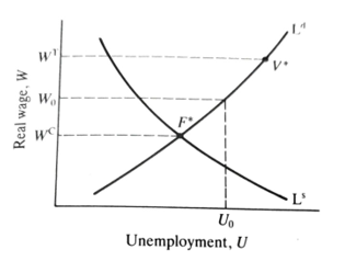
Figure 7.5 The wage bargain