Real Business Cycle Answers That Inspire Your Exam-Writing Skills
Don’t struggle with your next real cycle exam when we can help you prepare for it using these questions and answers. They provide a perfect way to answer exam questions for the best grade. The answers were prepared by seasoned economists from the best universities worldwide.
Explain the Real Business Cycle
The New Classical economists broke with a forty-year tradition shared by both Keynesians and Monetarists, in which both saw business cycles as being in some sense disequilibrium phenomena. To the extent this was true, the business cycle could (at least in theory) be smoothed by appropriate government policy. The New Classical vision, by contrast, is one of equilibrium business cycles. Random shocks bounce the economy into booms and recessions which (because of adjustment costs, say) tend to persist. However, agents are always optimizing - we are always in equilibrium. This was a radical departure; but what the new school kept from the old worldview is the notion that demand shocks are the driving force behind the business cycle. However, to some economists, this presented a number of puzzles.
Analyze Three Puzzles Associated with The Real Business Cycle
The first puzzle is about where the surprises are supposed to come from. In Chapter 4 we looked at three views of the model underlying the surprise supply function. Each of these seemed problematic. The most basic problem is that in the modern world, there are a great many individuals who are paid large sums of money either to generate economic information-for example, government statisticians or city economists- or to disseminate it -TV and other journalists, for example. A lack of information about prices drives the surprise models, but aggregate price inflation figures are routinely given prominence on national television immediately after they are published, with a relatively small lag after the period they refer to. Indeed, the retail price index is one of the most accurately known and speedily published of all economic statistics. Ironically, perhaps only the money supply is published with a shorter lag.
Another puzzle is an empirical one, to do with the movement of real wages over the business cycle. An omission from Lucas' list of business cycle characteristics is any discussion of the real wage. This is convenient for Lucas because it turns out that the real wage presents the biggest challenge for all demand-side stories of the business cycle. All demand-driven explanations of the business cycle-be they Keynesian or New Classical- a countercyclical relationship between real wages and output. For example, in the asymmetric information version of the New Classical story. predict that as prices rise the workers' perceived real wage rises (due to higher nominal wages), while in fact, the real wage falls. So employers demand more labor and output rises. Unfortunately for the model, there is very little evidence for such a relationship. Indeed, if anything the evidence is for a procyclical relationship-real wages tend to rise in booms.
A third puzzle is perhaps less worrying outside the economics profession. Realistic New Classical models must have some persistence in output, as discussed above. The explanations put forward (information lags, irreversible investment, and adjustment costs) deal with this very satisfactorily. Nevertheless, some economists feel uncomfortable with these ad hoc explanations.
Give A Solution to These Puzzles
One solution to all these puzzles was found in the 'real business cycle" approach. These models cut through the misperception problem (Puzzle 1) by arguing that it is not demand shocks that drive the business cycle, but ('real') supply shocks. These can be 'taste' shocks (changing consumer preferences), price shocks (like the fluctuations in the price of oil observed since 1973), or productivity shocks. Most models concentrate on the latter. Although the details can be complicated, the basic ideas are simple.
Firms use capital and labor to produce output, which can be either consumed or kept as a capital (investment) good for the next period. To keep things simple, pretend that households can be identified with firms -are self-employed producers, like farmers - so we can put the labor market to one side. Suppose there is a positive productivity shock. Households are now richer. Unsurprisingly, the optimal choice is to increase utility now by producing more output for consumption purposes and simultaneously holding back some extra output to use as an investment, thus increasing the size of the capital stock. What this second decision does is spread the benefits of the one-off improvement in productivity over time, just as consumers will save some or most of the 'transitory' increases in income in the permanent income model of consumers' behavior. This 'smoothing' effect means that random shocks will induce long-lasting changes in output, exactly what is required. This will be true even if productivity shocks are uncorrelated over time, as the capital stock lasts beyond the current period. Thus we have a perfectly consistent, optimal explanation of persistence. The theory also explains the procyclical movement in wages, as labor is paid its marginal product. It is also easy to explain the common output movements across sectors (point (i) made by Lucas on page 195 above) without appealing to economy-wide shocks, by noting that capital inputs come from other industries, providing a transmission mechanism through the economy. What is missing from this story is a convincing explanation of employment fluctuations, which are procyclical. This is true also for the New Classicists. The main idea to recognize is that for equilibrium business cycle theorists, fluctuations in employment reflect labor supply decisions so the rise in unemployment when employment falls is a purely institutional phenomenon. The unemployed voluntarily register for longer periods because they wish to work less. Given this argument, which convinces economists in the United States rather than in Europe, the focus moves to the elasticity of labor supply with respect to wages. In booms, as productivity rises, wages rise and more people want to work for longer hours. The awkward fact, unfortunately, is that (for men at least) the long-run elasticity is rather small; the supply curve for labor is pretty close to vertical.
One way to rescue the model is to appeal to intertemporal substitution in labor supply. The idea here is closely related to the permanent income hypothesis. Lucas and Rapping (1969) originally introduced the idea in the context of a natural rate explanation of the Phillips curve. When wages are temporarily high, workers will take advantage of this by substituting leisure across time and working more. So even if the long-run labor supply curve is vertical, there may be a positive short-run relationship. The problem with this explanation is that all the microeconomic evidence suggests that intertemporal effects are very weak indeed. An alternative approach is to allow interest rates to affect labor supply-workers work more when interest rates are higher, which boosts the return to saving (recall that interest rates are procyclical: point (vi) on page 196). Here also, the microeconomic evidence is against this hypothesis. Kydland and Prescott (1982) use a utility function that allows more possibilities for substitution, thus generating the required result. However, the evidence also rejects this approach.
This failure to explain the unemployment facts is a major problem with the theory. However, Lucas argues that the 'work of "equilibrium" macroeconomists is often criticized as though it was a failed attempt to explain unemployment (which it surely fails to do) instead of as an attempt to explain something else' (1981). This defense may not convince everyone, but if we accept the claim it implies we concentrate on the implications for output. The obvious way to assess the empirical adequacy of a theory is to set out its implications, construct an empirically tractable specification, and test the predictions of the theory against the data by standard econometric techniques. This has not been the preferred methodology for testing real business cycles, as essentially, they fail. Instead, models are constructed using plausible benchmark values for parameters and are then simulated to see if the results are comparable to the real data. This method has two major problems, one to do with statistical theory, and one more conceptual in nature. First, there can be no formal tests of statistical significance with this approach. Second, the whole process is driven by inherently unobservable productivity shocks. Originally, the variance of these shocks was chosen to generate an output variance equal to the actual data. It is obvious that this has a strong smell of circularity about it. However, there is no cast-iron alternative, although Prescott (1986) does try to estimate the shocks from a production function. Other empirical tests are available, though. One such is to look for permanent responses to temporary shocks, an idea which while not necessarily implied by real business cycle theory is certainly consistent with it. Technically, this follows if the output can be shown to have a 'unit root'. To understand this, take a simple example where the time series of output is given by:
Yt = α + βYt-1+ ԑt 0 ≤ β ≤ 1
where is a random error and ẞ is a parameter lying between 0 and 1. Begin with the case where β < 1. In the long run,' Y will settle down to a steady state value, say Y*. So if the 'long run' value of ԑt is zero,
Y * = α + βY*
= α / (1 - β)
A positive shock to Yt (ԑt >0) will have a short-run effect on Y which will persist, but in the end, the long run is unaltered. If β= 1, the whole picture changes dramatically. In this case,
Yt = α + Yt-1 + ԑt
or
Y₁ - Yt-₁ = α + ԑt
and the long run is simply not defined - there is no single long-run value towards which Y is tending. In this case, Yt is said to be 'non-stationary', or to have a 'unit root'. What happens if ԑt > 0 is that the effects of the shock persist forever. A 1 percent shock will raise output by a permanent 1 percent.
A technically complex debate began with the paper by Nelson and Plosser (1982), who argued there is a unit root in US output. Much of the problem is that in practice it can be extremely difficult to distinguish between a unit root and stationary processes close to but not actually at a unit root. The jury is still out and is fiercely arguing about this issue. the end, with regard to real business cycles, it may not be conclusive either way. Other models may also lead to unit roots-for example the insider-outsider model of Blanchard and Summers (1986) where employed 'insiders' act via their unions to maximize only their own welfare, ignoring the unemployed (see Chapter 5 for more discussion). This leads to the phenomenon known as "hysteresis' where output or unemployment is determined by its own history (see Cross, 1988b). Finally, many other models may generate behavior very close to and statistically indistinguishable from a unit root; for example.
The final piece of evidence does not rely on arcane econometric techniques or arguments about the predictions with respect to unemployment, or any other variable. Instead, it is the simple observation that while there may well be something in real business cycle theory, it seems very unlikely that it can be the major explanation of the three most recent recessions, beginning in 1974, 1979, and 1989. We have argued that two of these were affected by supply shocks, but these are not the stochastic draws of the real business cyclists; rather, they were massive blows from exogenous clubs. The effects were compounded by inept demand management. We would be quite incapable of explaining these episodes with real business cycle tools alone.
What Are Political Business Cycles?
A popular cause of economic cycles arises from the fact that economic policy is made by elected politicians. Such a policy may reflect the political objectives of the government. For example, to the extent that popularity is influenced by the state of the economy, a government may hope to improve its re-election chances by generating boom conditions just before a general election. A slump would presumably follow after the election. Such a pattern where booms coincide with elections is known as a political business cycle. One American author (Tufte, 1978) has gone so far as to argue that the cycles in the US economy are, more or less, all election-related. His evidence, however, is unconvincing, except for the case of the 1972 presidential election. Then, there was a substantial rise in Federal transfer payments (Veterans' benefits, etc.) just a week before the election. The most explicit theoretical case for a political business cycle relies upon the government riding the short-term Phillips curve. This argument is explicitly set out in Nordhaus (1975) and provides the basis for his claim that democracy causes inflation. Consider Figure 11.1.
The curves labeled P are short-run Phillips curves, with higher numbers reflecting higher levels of expected inflation. The curves labeled U are social indifference curves, the points along which will generate the same vote for the government-lower numbers reflect higher utility and a higher vote. The curve LRP is the long-run Phillips curve (Nordhaus takes it to be non-vertical, though this is not important so long as it is steeper than the P curves).
Each government finds itself on a particular P curve such as P2 The vote-maximizing strategy will be to run the economy at point B, which yields the highest possible vote. During the next period, however, since B is to the left of the long-run Phillips curve, the economy will be on a higher P curve like P3. This process will converge to a point like C which is on the LRP curve and, therefore, stable. This is sub-optimal because point A is the point of highest sustainable social welfare. The political process has generated higher inflation and lower unemployment than would be preferred. Readers may recognize this story; it is very similar to the inflation policy game set out in Chapter 4. In fact, much of the discussion there applies to the political business cycle.
As long as we are prepared to disregard the implications of rational expectations, it is easy to tell a story about cycles in this framework. Governments simply ride up the P curve to the highest U curve at election time. Then, after the election, they depress the economy - to the right of LRP so that they find the economy on the lowest possible P curve by the time of the next election. They then generate a boom again in time to be re-elected.
Plausible as this account may be, the evidence for it is remarkably weak. Even the proponents of this kind of 'political' view of policy (Frey, 1978) seemed to give up looking for electoral cycles in the targets of economic policy such as inflation and unemployment. Also, the evidence concerning the influence of the state of the economy on political popularity and voting is not at all clear-cut. It is certainly true that popularity can be significantly related to economic variables for some historical time periods. The problem is that the results have tended to be heavily sample-dependent. For other time periods, they are often substantially different. Particularly strong swings in coefficients are discovered when the results for the 1960s are extended into the 1970s. However, recent work by Price and Sanders (1993), who explicitly looked for structural change over the post-war period, revealed a stable relationship explaining popularity.
An alternative, and highly revealing, way of looking at the question is to ask whether the electorate can be fooled in the short run and whether the government acts as if it can. Asking the question this way focuses attention on the electorate's expectations, as well as on the current state of affairs. If electors are fully rational they will anticipate the post-election deflation and so there will be no benefit for the incumbent party in running a pre-election boom. Macrae (1977) incorporates expectations explicitly by distinguishing between a myopic and a strategic electorate. A myopic electorate only considers the current state of the economy whereas strategic voters have a longer time horizon. Macrae's results for the United States appear to show that the government assumed myopia from 1960-68 but strategic voting before and after. Applying Macrae's model to the United Kingdom, Chrystal and Alt (1981) conclude that 'the myopic hypothesis never significantly outperforms the strategic hypothesis'. And they are thus led to conclude that while on some occasions the government may indeed have manipulated unemployment with a vote loss or social welfare function in mind, there is no evidence that the desire to win the next election, as distinct from remaining in office as long as possible, was the motivation. Thus we must conclude that the evidence for a simple political business cycle in Britain is negative. There can be no presumption that the government manipulates the economy on the assumption of a short-sighted electorate.
What appears to be a more sophisticated attempt to incorporate political goals into economic policy analysis is provided by Frey and Schneider (1978). They develop what they call a 'politico-economic' model of the United Kingdom. There are two elements to this. First, government popularity depends upon certain economic variables. Second, various components of government expenditure are shown to be altered as a result of popularity, the time before elections, and the political makeup of the incumbent party. Chrystal and Alt (1981) show that if government expenditure and revenue are related to the trend of GDP virtually all the political factors drop out. The only significant political factor to remain is that transfers are higher under Labour than under Conservative governments, as might be expected. We must, therefore, conclude that electoral-cyclical and politico-economic explanations of budgetary policy in the United Kingdom are not well founded. A fuller discussion of these issues is available in Alt and Chrystal (1983).
Recently, however, political business cycles have made something of a comeback. As we observed above, the big problem with the earlier vintage described above was the implicit assumption that the electorate can be fooled that the government is smarter than voters. This is inconsistent with rational expectations. However, it is possible to generate limited business cycles even with the RE assumption.
There are two strands in this 'rational political business cycles' literature. The first is one of the opportunistic parties introduced by Sibert (1988). Political parties differ only in their competence. Competent parties get re-elected. The problem is that it is difficult to tell whether the parties are competent. The electorate relies on 'signals'. One such could be the ability to deliver goods and services at low tax revenues. So a government may 'cheat' by lowering taxes in an election year to fool voters into believing they are competent. Eventually, voters find out the truth: but then the election is past. The twist is that not cheating has a payoff, as the government can acquire a reputation for playing with a straight bat, which it can then cash in by cheating at the most advantageous time. It should be clear that this theory cannot explain regular business cycles, although it may well help us understand particular episodes in history.
The alternative is a 'partisan' model, where parties differ in their preferences. In particular, parties of the right are presumed to care more about inflation than parties of the left. This is public knowledge. In its original incarnation, as in Hibbs (1987), voters are irrational, and outcomes are determined by which party is in power, but in Alesina (1987) voters are rational. What drives the cycle here is that the result of elections is unknown before they occur. After an election, left parties will allow higher inflation than right parties, ceteris paribus. However, in a world of overlapping contracts, wages must be set prior to the election, and are done so on the rational expectation of inflation after the election, which will be an average of the left and right inflation rates, weighted by the expected probability of each party forming a government. In this setup, we would expect recessions after the election of right-wing governments (price expectations were too high) and booms after the left elections. Alesina (1989) has found there is evidence for this in post-World War II United States. However, this can by no means be the whole story-the timing of the Bush and Major recessions in the United States and United Kingdom were entirely wrong in the 1988-92 period. When the model was tested for the United Kingdom by Alogoskoufis et al. (1992) there was only a little evidence for the model in the pre-Thatcher era, and that hedged with qualifications.
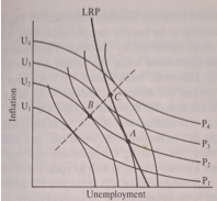
Figure 11.1 The Nordhaus model of the political business cycle.