Solving Macroeconomics Exams; 4 Essential Questions and Answer Examples
If you have an upcoming macroeconomics exam, these sample questions and answers can show you how to solve it excellently. Each answer deeply explains the question to maximize on the grade earned. The answers can also help you learn more about the new classical macroeconomics.
Explain Aggregate Supply in New Classical Macroeconomics
While most of the early arguments between Monetarists and Keynesians were about the determinants of aggregate demand (although see Modigliani (1977) for another interpretation), an important characteristic of the New Classical School has been their formulation of the aggregate supply curve. A fairly standard version of this would be:
Yt=Y*+n (Pt-t-1Pet) (4.7)
Where Yt is the level of output (national income) in period t; Y* is the constant 'natural' level of output2 associated with the vertical Classical aggregate supply curve; Pt is the price level or the rate of inflation in period t and t-1Pet is the price level or the rate of inflation expected to hold in the period t, when that expectation is formed on the basis of information available in period t-1. This says that there will be a fixed level of output except to the extent that actors make errors about prices. Notice that we can talk equivalently about inflation or the price level because
(Pt - Pt-1)-(t-1Pet-Pt-1)=(Pt-t-1Pet) (4.8)
and these variables are normally written in natural logarithms so that Pt-Pt-1 is the rate of inflation.
There are two somewhat different approaches in the literature which can be used to justify an aggregate supply curve of the form above. The first is due to Lucas and Rapping (1969) who underlies many of the New Classical explanations of the business cycle (see Chapter 11). It focuses explicitly on labour supply behaviour. Workers are presumed to have some notion of the normal wage, which may be thought of as the expected average wage. They have some flexibility as to how much they work, but in any given period more work means less leisure. Leisure yields positive utility, but so do the consumer goods they buy with their wages. In each period they have to decide how much to work, and they do so by comparing the current wage with the expected or normal wage. If the current wage is higher than the normal wage they will work more now in the expectation of taking more leisure in the future when the reward for working is expected to be lower. If the current wage is lower than normal they will take leisure now and expect to work more in the future when the reward is higher-in other words, there is intertemporal substitution. This behavior may reasonably be called 'speculative' labour supply. (Keynesian 'speculative' demand for money depends on comparing the current interest rate to the 'normal' interest rate.)
Thus, if the current wage is higher than expected more labor supply will be forthcoming and vice versa. The wage in question in both cases is presumed to be a real wage. The only way the price level (as compared to its expectation) enters into the Lucas/Rapping analysis is through its effect on the real interest rate. The real interest rate is important in its role as a way of discounting utility tomorrow into utility today. The expected real interest rate is defined as rt- In (Pet/Pt), where rt is the current nominal interest rate, Pet is the expected price level and pt is the actual price level. Lucas and Rapping argue that labor supply will be positively related to the expected real interest rate, and it is from this that labour supply would rise with (InPt –In Pet) for a given nominal interest rate. This connection must surely be extremely tenuous. It is hard to believe that labor supply is much affected by the real interest rate and it is far from obvious what the sign of that effect would be. It is even far from obvious what the effect of a change in expected inflation would be on the expected real interest rate. Indeed, the weight of the econometric evidence is against this kind of model.
While the precise link between the Lucas/Rapping analysis and anticipated price changes' is somewhat implausible, the spirit is less so. This is that a demand shock which is perceived to be temporary will have an effect on the current supply which is greater than that which would result from a permanent demand shift. This is because of the inter-temporal substitution of work into the period when demand is high and away from the (future) period when demand is (expected to be) lower. We shall return to this issue in the context of discussions of the business cycle below. Notice in passing, however, that the Lucas/Rapping analysis depends in no way on rational expectation; indeed, Lucas and Rapping themselves use adaptive expectations to determine the 'normal' level of wages and prices. What they do assume, however, is that prices and wages clear markets in each period. So changes in employment are perceived as 'voluntary' in the sense that everyone who would choose to work at current wage rates can do so. This is a source of some controversy which we shall return to below.
The second approach to aggregate supply is that found in Lucas (1972, 1973). Here the focus is directly on goods markets rather than on labor markets. Sellers are presumed to be located in one of a large number of "local" markets which are segregated, though within each market there is perfect competition. The local price is known for the current period, but the general price level across all markets is only learned with a lag. The problem for the seller is to decide how much to sell (and produce) by observing the current price. This is difficult because a change in price could reflect a shit in demand towards their own market (which requires a rational response) or merely a change in the value of money (which needs no response). Part of the decision, therefore, depends upon a single comparison of the curr local price with the expectation of the general price level for the same period If they are the same there is certainly no reason to change the supply. If they are different then the setter may wish to change the supply. However, the size of the response will depend upon perceptions of variability in the price level compared with the variability of relative price changes. It is here that rational expectations enter the scene since the actor is presumed to respond optimally to this price signal in the light of the knowledge of the true, probability distribution of price level changes and real demand shifts. If the variance of price level changes is high relative to the variance of demand shifts (they are assumed to be statistically independent), the price signals should be distrusted and the supply response should be small. If the reverse is true a change in the current price is more likely to reflect a real shock to which supply should respond. Therefore, η above (equation (4.7)) will be close to zero if price level changes have a high variance relative to the variance of real shocks. It will be significantly above zero if the reverse is true.
While providing a formal justification of the 'surprise' aggregate supply curve, this argument is not entirely convincing either, even though the supply curve itself has almost become 'conventional wisdom". One problem is that the restriction of information it requires is just as ad hoc as many of the alternative Keynesian stories such as sticky money wages. Why should a seller perceive the demand price for the product earlier than perceiving the general price level? It is quite possible that the reverse would be true. Aggregate information and forecasts are much more widely available than information on specific markets.
An alternative explanation of this supply curve is based on an asymmetry of information between workers and firms. This is the approach mentioned in Chapter 1 above. Demand for labour by firms depends upon the real wage where both the money wage and the price of output are correctly perceived. Labour supply depends upon the real wage. Workers perceive the money wage correctly, but their belief about the purchasing power of that wage depends upon their expectation of the price level. An unexpected increase in aggregate demand will lead to an increase in aggregate supply. Initially, prices will rise by more than money wages. Firms will correctly perceive this as a fall in the real wage and will demand more labour. Workers will incorrectly perceive a rise in the real wage and will supply more labour. The higher input will be associated with higher output, that is, greater aggregate supply. Whether or not expectations are rational, this effect can only be temporary as workers are unlikely to be fooled for long.
Again, this seems a somewhat tenuous basis for the theory of aggregate supply. Supply will only change if someone is tricked. However, some thought about the supply-side structure within which this result is derived will show why it must emerge in that framework. It is the characterisation of the economy which must be challenged to overthrow the result, not the internal consistency of the analysis itself. In an economy with one input and one output, there is only one relative price the real wage. The market-clearing real wage is unique (if both labour supply and demand depend on it) and that is all there is to it. Without more structure to the economy, there is no scope for real changes in output and employment, especially in response to nominal expenditures. This, of course, is why Keynes thought Classical economics to be unsatisfactory. The real problem is to explain why output and employment do actually fluctuate.
Is Policy Ineffectiveness Significant in The New Classical Macroeconomics?
One of the earliest claims made by the New Classicists was that ‘[macroeconomic] policy is ineffective’. Systematic demand management will have no real effects. This dramatic result created extraordinary controversy, and may indeed have temporarily set back the adoption of rational expectations because of the extremity of the conclusion. The first proponents of this idea, Thomas Sargent and Neil Wallace, now claim their seminal model was designed mainly as a vehicle to demonstrate the importance of taking expectations seriously; but even if this were the intention, their work was not interpreted in this light at the time. The supply function assumes great importance in this debate because the claimed ineffectiveness of systematic aggregate demand policy is crucially dependent upon it.
Consider Figure 4.1: the economy is initially at p0 Y*, with aggregate demand D0. The level of income Y* is the 'natural' level of output which is defined to be that sustainable in the long run. Any greater level will be associated with rising prices. The supply curve SA will be the response to an unanticipated shift in D. This is because with pe held constant, the curve of equation (4.7) has a positive slope with respect to pt However, as pet is revised upwards SA will shift to the left. With rational expectations, pet will not differ from p1 for any reason that could be predicted. Hence, if a shift in aggregate demand is anticipated all its effect will be felt in prices and not in the output. The economy will go straight from p0 to p₂, but Y* will not change.
In this framework any systematic policy reactions which involve shifting aggregate demand will have no real effect - at least where the authorities respond with a lag and they are not better informed than the actors. Consider again equation (4.7), which is modified only by adding a random supply disturbance eSt.
Y₁ = Y* + η (Pt-t-1Pet) + eSt (4.9)
Here and elsewhere, we assume that the random error eSt takes an average (or expected) value of zero, and is serially uncorrelated. Formally, E (et) and E (etes) =0(t>s). The price level can be assumed to be proportional to the money stock Mt, plus a random demand disturbance, edt:
Pt= α Mt+edt (4.10)
Let us suppose that the monetary authorities keep the money stock constant, except that they try to stabilize the economy by changing the money stock in response to deviations of the last period's output from the natural rate. They achieve this with a random error, emt.
Mt= β0+ β1(Y*- Yt-1)+ emt (4.11)
With rational expectations, actors will expect the price level to be proportional to the systematic component of the money stock (where we have used the assumption that E (et) = 0).
Pet. = α(β0+ β1(Y*- Yt-1)) (4.12)
The actual price level will also depend on the error in (4.11) and the demand disturbance.
Pt = α (β0+ β1(Y*- Yt-1))+ αemt+edt (4.13)
So the error in price expectations just depends on the disturbances subtracting (4.12) from (4.13).
Substituting this back into (4.9) results in the following:
Yt- Y*= ηαemt+ ηedt+est (4.15)
This says that the deviation of current real income from the natural rate only depends upon random disturbances and not at all upon the systematic component of the policy. This is essentially the analysis of Sargent and Wallace (1975), which leads to the conclusion that only unanticipated policy matters.
An obvious comment on this result is that if deviations from the natural rate (of output or unemployment) were really random then a stabilisation policy would not be necessary anyway. It is persistent deviations that have to be explained and, of course, corrected for. New Classical economists would all accept that there has to be persistence and, indeed, assume it (and discover it) in their empirical work. If they did not do so their case would hardly be credible. Lucas (1973), for example, writes his aggregate supply curve:
Yt- Y*t= η0 (pt-pet) η1(Yt-1- Y*t-1) (4.16)
where the term η1(Yt-1- Y*t-1) reflects persistence, though this persistence is not justified explicitly and must, therefore, be considered ad hoc. However, even though random shocks lead to sustained output changes this does not restore a role for systematic stabilisation policy, as repeating the above exercise with (4.16) instead of (4.9) will demonstrate.
One line of argument that will restore at least partial policy effectiveness is that of long-term overlapping wage contracts, a point made early on in the debate by Gray (1976) and Fischer (1977) (see also Taylor (1979, 1980)). This works by creating some stickiness in money wages and thereby allowing some temporary real wage changes which can be exploited by the authorities. Suppose, for example, that money wage contracts are set for two periods and the authorities continue to operate the rule (4.11). Wage contracts will presumably reflect price expectations over the subsequent two periods, but they cannot anticipate the systematic reaction of the authorities in the second period because this depends on the outcome in the first period which has not yet happened. Thus, aggregate demand policies will exert some leverage over aggregate supply in the short term. This effect will die out over time as the longest contract matures and money wages catch up with prices. But this approach is essentially ad hoc; we return to the issues in the next chapter.
However, even if wages are fully flexible, it soon became clear that the Sargent and Wallace case is very specific, and quite small changes in the specification, on either the demand or supply side, can reintroduce effective policy. Effectiveness will be restored if there are non-linearities in the model, for example, or if supply is forward-looking so that the next period's price is what matters. The issues are discussed further in Minford (1991) and Pesaran (1987).3
Turning to the evidence, the proposition that 'only unanticipated policy has real effects' seemed initially to gain powerful support from work by Barro (1977, 1978). On annual data for the United States for the period 1941-73, Barro showed that the unemployment rate was significantly affected by unanticipated money growth, but that it was either unaffected or affected perversely by actual money growth. Unanticipated money growth was measured as the difference between the actual and fitted values of an equation in which money growth depends upon its own lagged values, the deviation of the Federal budget deficit from normal and lagged unemployment. This is a mixture of a kind of reaction function and budget constraint. Unanticipated money growth has effects not only in the same year, but also in two subsequent years and, thus, illustrates the importance of persistence. Actual money growth has no significant negative effect on lowering unemployment, except a marginal one after four years. The overall fit was much worse than for unanticipated money.
Impressive as these results seemed, they were not in the end convincing. To begin with, the method of generating 'unanticipated' money growth is inconsistent with rational expectations. Information should only be used which was available at the time. There may be no relationship between the residual in 1948 of an equation estimated with a sample for, say, 1946-73 and the forecast error that would have been made in 1948 based only upon information available in 1947. My forecast for next year cannot be dependent on information that will only become available subsequently. Barro noted this but did not cope with it.
Simple as this point is, it opens a can of worms that has not yet been successfully untangled. The issues go beyond the question of empirical tests. The point is that although rational expectations offer a coherent theory of expectations conditional on a given information set, it offers no explanation of how this information is acquired. Perhaps we need a theory of learning to complement our theory of expectations. This observation has spawned highly technical literature exploring the changes that learning brings. The results tend to be specific to the model - sometimes learning makes the existence of a rational expectation equilibrium more likely, sometimes less. What is clear, though, is that no tractable ways of modelling learning have yet appeared. This is something of a disappointment, as the great advantage of the rational expectations (RE) approach was its apparent conceptual simplicity.
There is a further, very deep, problem with the tests. This can be appreciated by noting that the news that the rate of growth of money does not explain unemployment will be quite happily received by Keynesians, Monetarists and New Classical economists alike - but for very different reasons. A wide variety of models may yield the same predictions. Going beyond this, the evidence that only unanticipated money matters is at first sight rather harder for a non-New Classicist to explain, until it is realised that this is consistent with a completely different scenario. Suppose the authorities are pegging interest rates rather than controlling the money stock (fixing the exchange rate will do just as well). Real disturbances will then cause monetary changes rather than vice versa. In so far as the real disturbances are uncorrelated with earlier monetary growth, the current monetary change will be unpredictable by any monetary rule. Her course, causation runs exactly in reverse and so constitutes a very kind of explanation. This substitute explanation must have some prima facie plausibility in light of the widespread practice of stabilising bo interest rates and exchange rates in the bulk of the sample periods studied so far, though this evidence is at least consistent with the New Cla view. So quite disparate models predict the same qualitative results.
Pesaran (1982, 1987) showed that while the method employed by Bam could show the data were consistent with the RE/ineffectiveness model, could not reject the Keynesian model, for the simple reason that there are well-defined Keynesian models with 'observationally equivalent' specifications, as discussed above. A better approach is to test the RE and surprise supply parts of the model separately, and then to test the implied cross-equation restrictions. Attfield, Demery and Duck (1981) find that the restrictions are (just) accepted by this method; but the observational equivalence problem remains. What is really needed is a well-defined (Keynesian) alternative against which the model may be tested. When Pesaran used such a framework, he found the Keynesian model output- formed the New Classical version.
Perhaps unsurprisingly in view of the theoretical arguments against ineffectiveness, the weight of the evidence is now opposed to the proposition. However, there is more evidence from individual survey data supporting rational expectations in (for example) consumption decisions. and financial markets appear to act in a way that is at the very least extremely close to full rationality. This is quite fortunate for the theoretician, as there is no obvious alternative to the notion of rational expectations. It is almost as basic as the notion of maximising behaviour. but, at the risk of labouring the point, this does not automatically support the New Classical doctrine of policy ineffectiveness, which is a joint hypothesis.
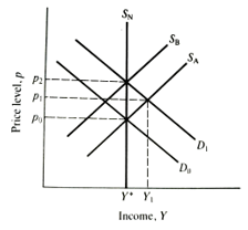
Figure 4.1 New Classical aggregate supply.
How Do Policy Games Play Out in The New Classical Macroeconomics?
Perhaps the most profound insight that the New Classicists brought to macroeconomics was that agents will try to predict the actions of governments. As we saw, one of the initial consequences was the ineffectiveness proposition, which in the end did not stand the test of time Once we realize that agents are trying to predict the actions of government the nature of our models shifts in a fundamental way. The point is that behavior will in general be affected by one agent's guess (conjecture) of what the other will do. Models of this kind, where agents have to react to other agents on the basis of their conjectures about the other party's behavior, are known as 'games. It turns out that the implications for macroeconomics go very deep. What is more, this insight helps us to understand the operation and formation of key economic institutions in our society, such as the Exchange Rate Mechanism of the European Monetary System, or the Bundesbank in Germany.
To understand the issues, we will first look at a one-period game between the public and the government. The fact that the game is only for one period is not as severe a restriction as one might imagine, as we will explain below. The game is about inflation. The government chooses the level of inflation, given what it believes the public's expectation of inflation will be; in turn, the public chooses its expectation, given its belief of how the government will act. We assume that both players have rational expectations, so an equilibrium can only exist if both parties' expectations about the other are correct.
Figure 4.2 shows aggregate supply in the short and long run. The only difference between this and the setup in Figure 4.1 is that we have inflation on the vertical axis, not the price level. As equation (4.8) reveals, the two ways of drawing the diagram are perfectly equivalent. The short-run supply curves are all drawn for different levels of inflation expectations. Only where they cut the long-run supply curve S, are expectations correct; thus all rational expectations equilibria must be at output Y*.
Suppose that the public dislikes inflation. If so, then the best possible equilibrium is at point A, where we enjoy zero inflation and the long-run level of output. If both government and the public have the same preferences, the game is trivial. Both parties will want to be at A; as it is in both parties interest to be there, this is what both will expect, and A is where we will end up. However, suppose that the government, while disliking inflation, would also prefer to have output higher than Y*. One way of formalising this is to define a government cost function, C:
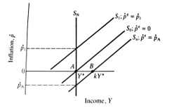
Figure 4.2 Short- and long-run supply curves.
C=aṗ2+b(Y-k Y*) ²; k>1 (4.17)
The government cost function C is equal to times the square of inflation ṗ plus b times the square of the deviation of output Y from kY*.
For simplicity, C is defined as a quadratic. The function puts a specific cost on deviations from either zero inflation or the target output level, kY*. As k is greater than one, this target exceeds the long-run rate. The function is smallest (actually zero) when inflation is zero and output is equal to kY* say, at B. As can be seen from the diagram, in order to get to B, the public would have to expect inflation to be negative (so that we were on Sa). The problem with this is that the public is assumed to know what the government's preferences are (i.e. equation (4.17)), so if inflation were expected to be ṗA they would expect the government to set inflation at zero; but this is greater than ṗA- so an equilibrium at B is inconsistent with rational expectations. The government could promise to fix inflation at ṗA of course, but no one would believe them. In the jargon, the promise would not be credible. B is the government's first best position, but it is unattainable. Given this, the second best position would be A where the government meets its inflation target, and we are also at the long-run level of output. Unfortunately, this is also unattainable. Suppose the public expects zero inflation, so we are on S0 in Figure 4.3. We have now sketched the government indifference curves' implied by equation (4.17). They give the trade-off between inflation and output; ceteris paribus, (for positive inflation) lower indifference curves are preferred. Clearly, if ṗe is zero (so we are on S0), then the government will want to set inflation at the level corresponding to point C on the diagram, where the indifference curve is tangential to the supply curve. This is the best the government can do, given the short-run supply curve. Inflation will again be at a higher level than the one expected. C could be called a 'cheating' equilibrium, as it requires the government to fool the public into thinking inflation will be lower than it actually turns out to be. There is a whole set of such points that minimize the cost function given the public's expectations; this is the government's reaction function, though there is only one position where the government's optimal inflation choice (given the public's expectation) is identical to the actual expectation (itself formed given the public's knowledge of how the government behaves). That point is where the government's indifference curve is tangential to a short-run supply curve and is on the long supply curve - where the reaction function crosses the long-run supply curve, at E5. So this unique point, E, characterized by high inflation, is the only possible rational expectations equilibrium.
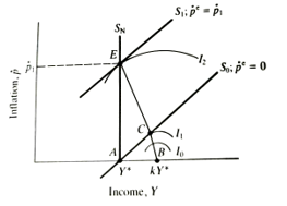
Figure 4.3 A policy game.
Thus we have an apparent paradox. If the government and the public could somehow agree to be at the zero inflation point A, both would prefer the outcome to the high inflation outcome E (which is at the same level of output, and therefore unambiguously worse). Somehow, this obviously desirable outcome cannot be achieved. Why is this?
The basic problem stems from the timing. In effect, the public chooses its expectations before the government sets inflation. As there is always an incentive for the government to cheat, the public always assumes it will do so, unless inflation is expected to be so high that there is no incentive to cheat (as at E). If the public and government could somehow make their moves simultaneously, there would be no problem. However, this is not possible. The general problem is time inconsistency. The rationale for this phrase is that although ex-ante it is rational for (in this case) the government to go for zero inflation when time has moved on and the public has irrevocably set its expectations (via wage contracts and the like), the world has changed, making it optimal to cheat. It is as if the structure of the problem changes with the passage of time. Although this idea has been extant in dynamic programming for some time, it was Kydland and Prescott who first pointed out the dramatic implications for macroeconomics in 1977.
Can We Fight Time Inconsistency in New Classical Policy Games?
Yes, there may be ways out of this bind. One way is to repeat the game an infinite number of times. Barro (1983) showed that in this case, a government may be able to acquire an anti-inflationary reputation which can be sustained in equilibrium. The idea is that the public can impose costs on the government by 'punishing' governments which spring inflation surprises by setting their inflation expectations high. While this sounds arbitrary, it is possible to show that this is in fact an optimal strategy for the public. This punishment can make it optimal for the government to keep inflation low (though not zero). The key idea, to which we return below, is that an outside force is imposing extra costs on the government if it lets inflation rise. This makes it in the government's own best interest to control inflation. So low inflation equilibria are possible. The problem, however, is that repeating the game 100, 1000 or even 10,000 times is not enough. In finite cases, no matter how many times the game is repeated, there is always a last game when the government has the incentive to cheat. As this effectively wipes out the last period, the last game moves back to the period before the last (as we know the government will try to cheat in the last game and cannot keep its reputation). However, in this new last game, the government will again have an incentive to cheat, so the next-to-next last game now becomes the effective last game and so on. All finite games unravel to the current period.6 Only in infinitely repeated games can reputations be sustained.
As no government in history has yet been seen to last forever, this is not a very helpful approach. However, Backus and Driffil (1985) showed that uncertainty can help. If there are two types of governments - one tough on inflation and one soft - then it may pay the soft type to pretend to be tough By doing this they can build up some anti-inflation credibility which may be useful to cash in later, possibly in a severe recession, or just before an election. So if there is uncertainty - as there surely is - then low inflation equilibria become more likely. This approach has a distinct appeal to the observer of the recent economic scene in Britain. It is certainly possible to tell a story about the Conservative administration that follows the line set out above. Between 1979 and 1984 the Government undoubtedly acted as If it were tough on inflation, allowing unemployment to rise to record levels at an unprecedentedly rapid rate, and presiding over a proportionately greater decline in manufacturing output between 1979 and 1981 than between 1929 and 1931. Yet in 1986, with inflation screwed down to 21/2 per cent, the pound was allowed to float down and the scene was set for a tax-cutting budget before the 1987 election. These policy choices undoubtedly contributed towards the subsequent unsustainable boom and inflation of the late 1980s. We shall have more to say about the political business cycle in Chapter 11.
There may be more direct routes towards a low-inflation world. The basic problem facing governments is acquiring some anti-inflation credibility. As governments are never held to the implicit contracts they form with the electorate (manifesto pledges are not enforceable in the courts), this is difficult. The key ways that have been proposed to circumvent this problem all involve tying the government's hands, in Giavazzi and Pagano's (1988) graphic phrase. Paradoxically, by deliberately restricting the scope for independent action, it may be possible to achieve better outcomes. The issue is one of 'pre-commitment to a policy One way of doing this is to make the central bank, the institution that is directly responsible for monetary policy, constitutionally independent of the government. This is the German model, where the Bundesbank is not only independent but also has as its overriding aim the explicit maintenance of price stability or zero inflation. When the German government pursues potentially inflationary policies, the Bundesbank will step in to raise interest rates to offset this. That it will indeed act in this way has been dramatically confirmed during the process of German reunification, where, arguably, some distinctly imprudent policies were pursued by the German government. Despite intense international pressure, the Bundesbank kept interest rates at such a high level that the domestic tensions in some ERM members like Britain and Italy came close to destroying the system; indeed, it is not clear at the time of writing that the ERM will survive.
The ERM effectively ties participant currencies to the Deutschmark (DM) Historically, German inflation has been very low; indeed, in 1986 German prices actually fell. So locking on to the DM is a way of imposing an external discipline. There is nothing strictly to prevent governments from allowing inflation to rise, but if they do, exports become uncompetitive, manufacturing suffers, and unemployment rises; these are unwelcome costs that make governments unpopular. So ERM membership imposes extra costs on governments when inflation rises. This is just what is needed to make low-inflation equilibria possible.
The problem, as shown by the dramatic events on 'Black Wednesday"7 in September 1992 when Britain was summarily booted out of the ERM by a tidal wave of speculative pressure, is that the need for credibility is simply pushed sideways. Before ERM entry, there was a problem maintaining a credible anti-inflation stance; after entry, the problem was to convince observers that continued membership in the teeth of a deepening recession at a time of high real interest rates was itself credible. We return to the wider issues of international policy coordination and exchange rate regimes later in the book.