Get Answers to These 10 Questions Regarding Econometric Demand Forecasting Exam Preparation

This chapter outlines the managerial economics approach to forecasting demand, using econometric methods to produce and test a model of customer behaviour. Econometrics is a subject in itself beyond the level of our present approach. The aim here, as in other chapters, is to place the techniques in context, showing the main assumptions made, the main achievements, and some of the problems. We also aim to help you take your econometrics exam. We have economics exam help services that guarantee you a top performance for all seasons. With this in mind, we start by outlining what this approach needs and how it draws on economics and statistics. The single-equation linear model (the most basic econometric demand model) is then outlined, stressing its assumptions' restrictive nature. We then look at the problems arising when we use this powerful tool in real situations.

What Is Econometric Demand Forecasting, And What Are Its Major Components?

An econometric demand forecasting model is one where we have statistical evidence for the model's parameters. It is called econometric because the evidence has been obtained using methods evolved by the still-developing combination of economics and statistics called econometrics. To develop an econometric model, we need four components or inputs:

A priori knowledge of the model;
Knowledge of probability theory;
A statistical technique that fits equations to data; and
Computing power to do the calculations.

Let us examine each of the inputs in turn to assess their contribution.

A priori knowledge

We need an initial model with which to start our model-building. We can build it up in stages, as we saw earlier in the book, first identifying likely causes and then the direction of the relationship concerned. Economic theory provides an easy starting point for many products by suggesting income and price as variables. Likewise, the crucial ledge of the professionals working in the particular market will confirm or deny certain hypotheses and suggest alternative causes of changes in demand; from this, a priori knowledge model tests against data from the past.

Probability theory

Knowledge of probability theory is needed because we can only test our model against a sample of all possible situations. We need probability theory to tell us how much confidence we can place in the results. How likely is it that our sample of years could give us a result unrepresentative of the 'real' forces at work in this market? We are still finding out some of the properties of the small samples (20-30 observations) that we often have to work with in forecasting. Probability theory tends to tell us not that we can be very confident that we have found the 'true' cause and effect relationship but that we should be either cautious or very cautious!

Ordinary least squares (OLS). This is the name given to the most common technique of fitting an equation to data. It can be explained using Figure 13.1.

If we have a scatter diagram of observations, such as in Figure 13.1, we could try to represent them by a continuous line. This line could be a curve or a straight line. Most of the work up to now has been with straight lines, and as the principles are the same in both cases, we, too, will use the example of a straight line. If we do this, of course, we are accurate. We assume that linear regression is adequate for the level of e required.

Table 13.1 Least squares: calculations

Deviation of the observed demad

Income	Observed Demand	From A	Squared	From B	Squared
8,000	8	0	0	2	4
9,000	5	4	16	2	4
10,000	9	1	1	1	1
11,000	10	1	1	1	1
		6	18	6	10

There are several ways it could be done, but the one chosen in ordinary least squares is to square the deviations. Thus the chosen line is the one with the least sum of the squares of the deviations. The calculations are given in Table 13.1. Line B is preferred using the sum of squares method. We can make two obvious observations on this result. First, just recording the deviations' signs and summing them would have given the same result: A totals -6 while B totals +2 only. Secondly, there is likely to be a better line than B. Reading a standard statistics text will tell you how to find it. Squaring deviations would seem an unnecessary complication, but it has advantages when we are comparing two or more scatter diagrams (or samples). It then produces a lower sum of squares for 'compact' scatters than for 'dispersed' ones. So not only does fitting the 'best' line in any example produce a lower sum, but it also enables us to compare the likely accuracy of different forecasts. In samples with high sums of squares in the line, the calculations will be inaccurate on many occasions. It will represent an average, a compromise rather than a close approximation.

What Are The Advantages Of Using The Ordinary Least Squares (OLS)?

There are two major advantages to using ordinary least squares; it is easy to compute, and their properties and drawbacks are well known. Both of the points are discussed further later.

Computing power

We mentioned computing power as an input because the advent of calculators and computers has made statistical analysis much easier. Previously only research workers could do the kind of statistical investigations that could be done on relatively cheap calculators. This has its danger, and the rest of this chapter points out some dangers of rushing where econometricians fear to tread.

The Single-equation Model

The simple model we shall use in this chapter as a reference point is called the single-equation model. Like many other models we have used, it is often used without realizing its limitations and certainly without stating them.

Explain Major Assumptions Made Regarding the Listed Models

The following are the major assumptions made about models which are tested using the ordinary least squares technique:

If we express our model in one equation, we must be sure that the variable on the left is the dependent variable and the variables on the right are independent. In other words, we are assuming (in the single equation forecasting model D= A+BY+cP):

D is caused by Y and P and does not cause them. Y is not caused by either D or P.

P is not caused by either D or Y.

D is not caused by past values of D

If we make these assumptions, we can assume certain relations between the data we use to test the 'true' relationship. If we cannot make the above assumptions, problems ensue and the single equation method using ordinary least squares can not be used with any theoretical justification.

State Practical Solutions to the Assumptions of the Models

In practice, there are three solutions to the problem of the above assumptions not being met: to ignore the theoretical problems and to produce solutions embodying new techniques, expertise, or judgment. We shall not go into these or use solutions in any detail, but examining the problems will suggest how they are often solved in practice.

What Are the Limitations of Using the Single-Equation Model?

Real data very seldom conform to the ideal data required for this model. The problems which arise are usually considered under the following factors:

The nature of data and models

The models we may wish to test are often static, i.e. they refer to values of variables in a particular period, but real markets are essentially dynamic. This produces many problems because we can safely assume that many variables are caused, in part at least, by the previous values of other variables (which is fairly easy to incorporate into the model) and by previous values o themselves. Much forecasting work is done with time series, which exhibit strong evidence of serial correlation. Sales of most products are close to those in previous periods, and it becomes a matt of judgment to decide whether this is because of habit (the dependent variable is caused by itself) because what caused high sales last month exists and will cause nearly as high sales this mo too. There are two ways in which we can attempt to get over this problem: one is to combine series and cross-section data (defined below mitigate the serial correlations, and the other is to use a time interval as long as, say, a year, in which all the lagged effects can be assumed to have worked themselves out. Both methods work but introduce other problems, as we shall see later in this chapter.

Data problems

Even if we are happy that our model is close to the type of cause and effect which occurs, we may still have problems with data, which we can consider under the headings of quality, quantity, and outliers. We meet the quality problem, particularly with price data, which is notoriously unreliable. The further reading by Morgenstern contains many examples of how errors arise in economic data, some very amusing, if not tragic! We often cannot obtain the particular data we need, say a particular price series, so we have to use a proxy variable, another price series, as a substitute or proxy.

Fig.13.3 An outlier

If we have good-quality data, we may still have the problem. Ideally, we need over 200 observations to operate the best-known aspects of probability theory. If we have fewer data, it is difficult to be confident that our sample represents the 'real' relationship at work. However, it isn't easy to obtain long time series for products. Even when available, their quality is low because the product specification has changed over time. Large numbers of products enter and leave the market every year, and thus our data cannot be long-term. The solution is to simultaneously use cross-section data, i.e. from several markets or customers. This raises the quality problem again.

Shall We Assume The Markets Are Similar, Or Shall We Introduce Another Variable Into the Equation (A Dummy Variable) To Account For, Say, Climate, Or Ethnic Factors?

Some econometricians are now meeting this problem directly by exploring and clarifying the properties of 'small samples', the twenty or thirty observations that are often readily available in many situations.

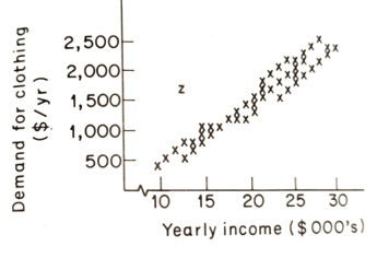
The last problem with data is how to deal with data that are outliers. If we collect data from a questionnaire, we often see a pattern like that in Figure 13.3 with one or more 'outliers' like z.

If we include the observation in our calculations, it will pull the whole line towards it. So, are we justified in excluding it? The answer lies in knowing more about the observation. It may be a mistake, a coded reply, a punching error, etc., which escaped our data-vetting system. If so, it should be disregarded.

Alternatively, it may be genuine but not representative; it may exist but play a larger part in our sample than in the total population. This poses a more difficult problem with three obvious solutions: (i) discard it as over-representing a particular type of consumer or market; (ii) reduce its significance by weighing it by its weight in the population as a whole; and (iii) include it, but mention its biasing effect in footnotes.

The third type of outlier is the hardest to deal with, being both genuine and representative. This is a customer or market which is eccentric. Marketing professionals often solve this problem simply by disregarding it as a special market of its own and thus not relevant to the main study. Cavalier though this seems to some 'scientific' observers, it serves to produce more easily communicable results. Moreover, the extra variable needed to 'explain' the behaviour of the eccentric consumer may not be worth its cost. Forecasting is, after all, an economic activity - the marginal cost must be less than the marginal revenue!

The identification problem, one of the classic early statistical studies of demand (Working, 1927), used time series for the price and demand for pig iron in the late nineteenth century. The result was a curve like that in Figure 13.4.

Establish the Identification Problem for the Demand and Supply Curves

One of the classic early statistical studies of demand (Working, 1927) used time series for the price and demand for pig iron in the late nineteenth century. The result was a curve rather like that in Figure 13.4.

This might lead us to the conclusion that demand rose when the price rose, the opposite of the usual relationship. However, the obvious question is whether we have a demand curve before us. In demand and supply analysis, actual prices are where demand and supply curves cross, so any one of the observations would be on both the demand and supply curves for that year. We would only trace the demand curve if it did not shift and the supply curve did.

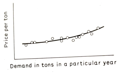
Fig 13.4 Demand curve for pig-iron

What is far more likely is that the supply curve for pig-iron shifted a little over the years, but demand was affected by the rising output of steel, railways, ships, etc. Figure 13.5 illustrates this.

This historical digression is included because one of our main problems in analyzing data is identifying the relationship that we have calculated or plotted. To plot the demand curve for a product, we need to find a variable (shift variable) that will shift the supply curve. Again, going back to the introductory economics, technology will shift demand curves. Remarkably, there is a connection between the simple graphical analysis above and the complications needed to analyze some markets that cannot be tackled using single equation methods. In both cases, it is the existence of shift variables that solves the problem of identification.

What Is The Basis Of The Specification Problem Established In The Equation?

The specification problem lies in knowing whether the right variables have been included on the forecasting equation's right-hand side (RHS). We can summarize the problem by saying there must be enough variables and not too many. First, how can we ensure that there are enough? As usual, the answer lies in combining economic and statistical knowledge. Suppose we use methods to analyze some price and demand data and find that it shows a positive relationship. In that case, our economic knowledge tells us that D = a + bP is insufficient to explain what has happened.

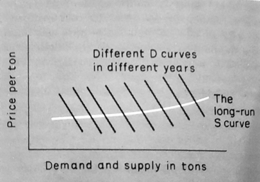
Fig. 13.5 Long-run supply curve for pig-iron

If demand rose while the price rose, another variable is likely to have caused it. Thus we change our model to D= a + bP + CY assuming that income (Y) has increased and demand to increased despite the price increase.

Give an Example Explaining the Effects of These Variables

Deciding when we have too many variables in the RHS is a little more difficult. For instance, we assumed that car ownership was based on price, income, and educational level. We might easily put data for different countries into a regression program and find results like D = 0.1 x Population-0.2× Price +0.013 x Y + 0.06 x years of education. This looks interesting until we realize that there is a very close relationship between income and education. We speak of these two variables as being mutually correlated or collinear. They break one of the initial rules of the linear regression model that the RHS variables should be independent. If collinearity exists, the parameters (calculated by the regression program) will be meaningless, and the usual solution is to discard all except one of such variables. This is another reason why many forecasting equations feature income: it is strongly correlated with so many variables that it often supersedes more obvious variables in forecasting models.

When Does The Problem Of Simultaneity Occur?

When one of the RHS variables is affected by the 'dependent' variable, then we have the problem of simultaneity. For example, if we have the equation = an x bp + cy but know that the price will differ when demand changes, then we have a problem. We need to know the relationship between price and demand; in other words, we need at least one other simultaneous equation to describe the market in question. For example, in functional form:

D= f1 (P, Y)
S= f2(Y)
P = f3(S, D)
Y = some value

There are three solutions to the problem of simultaneity. First, we can select only problems where single equation approaches will work, i.e. where all the RHS variables are genuinely independent. Allan discusses a possible example in further reading. The second approach is to collapse all the simultaneous equations into one 'reduced form' equation, ensuring that all the RHS variables are genuinely independent. The third approach uses more complex estimation techniques than ordinary least squares.

Technique bias

Any estimation technique c can be assessed for bias, consistency, and efficiency. It is said to be efficient if it gets results closer to the 'true' parameters than other techniques. It is consistent if the larger the sample, the nearer to the 'true' parameters it gets. Finally, it is said to be unbiased if it gives the 'true' value of the parameters as opposed to consistently or underestimating them. OLS is biased if the data do not conform perfectly to the linear over or regression model assumed (i.e. dependent variable forecast by independent variables). Thus it produces nonsense results in situations such as the pig-iron one we mentioned above or any situation where its assumptions are violated.

Thus we have the overwhelming problem of an estimator who is biased in almost all the cases we are likely to find in forecasting, and managerial economists have tackled this in three ways:

ignoring the problem, which is inexcusable.
finding cases where it is accurate enough.
using in- increasingly sophisticated econometric methods.

Perhaps the most encouraging way to end this chapter is to reiterate my belief in mixtures of techniques for solving problems. Econometrics is not the answer to forecasting, but it is a very useful addition to the forecaster's toolkit.