Fall 2022 Final Exam Solution on Constructing a Probabilistic Model Exam. SPSS at the University of Toronto.
Exam Question: using charts, distinguish the types of probabilistic models, and establish their effects in the business sector.
Probabilistic Models
Probability distributions
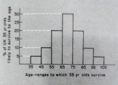
Fig. 3.1 Normal distribution: 'life-table"
Thus if we believe that a variable has a probability distribution that is 'normal', we can describe it using only two parameters. If we need to set up a computer simulation, the values of the variable can be generated, on some computers, once we have defined the parameters. The values the computer generates will appear 'random', but they will belong to the normal distribution and eventually produce the shape shown in Figure 3.2.
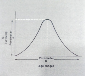
Fig. 3.2 Normal distribution: parameters
The rectangular distribution
We often need numbers in simulations with even simpler characteristics than the normal distribution. For instance, we may think that any of the four outcomes is equally likely. This means that the probability distribution looks like Figure 3.3 and is often called rectangular. We shall use this very simple distribution in the simulation later in the chapter. It is valuable for two main reasons, it is very easy to use, and many business phenomena are of this kind. They come in whole numbers (customers/cars/ tankers), and we have no way of knowing that any one number is more likely than another.
Computers and random numbers
Most computers have the facility to generate what are called random numbers. Being machines, the numbers are, of course, not truly random, merely generated in a way that is not immediately obvious to the user. There is a simple way to test how 'random' your computer is by using the program in Appendix A. This takes the first digit of the number supplied by the computer and counts how many times each digit occurs. If the numbers were truly random, each digit should occur with the same frequency.
If we run the program first for 10 numbers, then 100, then 1000, etc., the frequency distribution tends to become rectangular. The tendency of the events to approach the theoretical frequencies is known as the law of large numbers. It explains why events can appear to be random and still be forecasted over a large number of occurrences. Our 'life tables' have this characteristic: we cannot forecast individual life-expectation, but the average for many people could be very accurate.
This clarifies the notion of risk: an individual is uncertain about his life expectancy, and an insurance company with many policyholders is in a risk situation. Overall the company cannot lose if the average life expectancy, and the resulting premiums, have been accurately calculated.
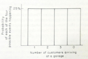
Fig. 3.3 The rectangular distribution
Decision Theory
When we deal with static probabilistic models, we often use concepts collectively known as decision theory. For this, we need some additional vocabulary. Let us consider a simple example: a firm attempting to locate production facilities in one of three areas. In many ways, the areas are competitive but under different circum- stances. One area will be most competitive if the home market grows rapidly, another if export markets grow, and the third if world inflation is particularly severe. However, the firm does not know which of these three possibilities is most likely. (For simplicity's sake, we assume only one of the three possibilities will occur.) So it might list the results of locating in each of the areas (A, B, and C) if each of the three scenarios,
Fig. 3.1 Decision theory: payoff matrix
| Different locations | Effect on the firm's profits under different circumstances($m) | ||
|---|---|---|---|
| H | X | F | |
| A | 10 | 1 | 6 |
| B | 0 | 12 | 2 |
| C | 2 | 3 | 10 |
Home market growth (H), export market growth (X), and rapid inflation (F) occur, as in Table 3.1.
The figures in the boxes, the effects on the firm's profits, are termed payoffs, the different locations are called strategies, and the different scenarios are called states of nature. The firm is thought of as playing a game against nature and trying to ensure the best possible outcome, whatever might happen. It is presumed that it can decide which payoffs are best and put them in order. In our example, if the firm's main aim were profit, the order of its preferences would be obvious. If we are to use decision theory, we need to know one more thing about the firm, rather surprisingly, its psychology! We need to know whether the firm is optimistic or pessimistic when making decisions. Does it act expecting the best or the worst; is it a gambler or very cautious? We formalize these characteristics of the firm's decision-takers into a decision criterion.
Decision criteria
Several possible decision criteria are used when we do not know what will happen. (Observant readers will notice that we are talking about uncertainty rather than risk; decision theory was originally developed to deal with uncertainty. However, its use in situations of risk will soon become apparent.)
A pessimistic decision taker would tend to assume the worst might easily happen and thus choose the strategy whose worst outcome was better than the other strategies' worst outcomes. The best outcome of a strategy is called it's maximum, and the worst outcome it's minimum; thus, the pessimistic decision criterion involves choosing the strategy
Fig. 3.2 Decision theory: expected values
| Payoffs under different states of nature($m) | Average payoff($m) | |||
|---|---|---|---|---|
| H | X | F | ||
| A | 10 | 1 | 6 | 5.67 |
| B | 0 | 12 | 2 | 4.67 |
| C | 2 | 3 | 10 | 5 |
With the highest minimum. It is called the maximin criterion. Applying this criterion to our example would entail choosing location C.
An optimistic decision-taker would be more likely to look at the maximum of each strategy when comparing them. This criterion of choosing the strategy with the highest maximum is called the maximax criterion. This criterion would choose location B in our example.
Other possible criteria might involve some form of compromise between these two extremes. However, one criterion provides a link with situations of risk, where we know the probability of certain things happening. It is called the Bayes or Laplace criterion, or principle of insufficient reason.
The Bayes criterion
There is a long intellectual history to the idea that if you do not know the probability of something occurring, you should assign equal probabilities to all the possible outcomes. We commonly do this, and the Bayes criterion merely formalizes what is almost automatic. However, assigning a probability to an event can transform it from uncertain to risky. In our example, if we assume each of the three states of nature is equally likely, then we can produce an average payoff with equal weights to each of the original payoffs, as in Table 3.2.
We have called the 'average payoff of a strategy' its expected value. Thus a rational firm that did believe each of the outcomes (H, X, and F) equally likely, would choose strategy A.
Table 3.3 Decision theory: calculating expected value
| A: 0.5 X 10+ 0.1 X 1+0.4 X 6 = 5+0.1+2.4 = $7.5M |
|---|
| B: 0.5 x 0+ 0.1 x 12+0.4 x 2 = 0+1.2+0.8= $2.0m |
| C: 0.5 x 2 +0.1 x 3+0.4 x 10 = 1+0.3 + 0.1+ 4 = $5.3m |
Expected value
Thus the expected value of a strategy is the payoff under each state of nature multiplied by the probability of that state of nature. This means that when we have information about the probability of different 'states of nature', we can incorporate this in our calculation, which will very often affect the decision. For instance, a rapid inflation rate was expected if neither the home nor export markets were expected to grow. We would assign a value of 0 to the probabilities of H and X, and 1 to the probability of F. Project C would then be chosen. Table 3.3 shows what would happen if we gave a 50% probability to H, 10% to X, and 40% to F (the probabilities must always be 100% or 1). Thus we can calculate an expected value of the payoffs of different strategies when we know the probabilities of the different 'states of nature'. When we do not know the probabilities of future events, we have to rely on the Bayes criterion, or principle of insufficient reason, as it is often called and assign equal probabilities to each possibility. However, dealing with 'uncertain' events is more unusual than calculating expected values for risky ones, and the other criteria mentioned are often used.
What if we have a dynamic model in which we only know the probabilities of events happening? Can we analyze it? The short answer is that it is possible with some models to provide solutions. However, almost all dynamic models can be used as 'simulations', and we now turn to the simulation of a dynamic probabilistic model.
Queuing problems
Many businesses have problems that have been described as queuing problems. They involve the customer arriving for some service at irregular intervals and the supplier having to decide how many service points to provide. For instance, oil terminals have to provide the right number of tanker berths, hire firms with the right clothes/cars/excavators, and post offices with the right number of assistants at the counter. The essence of the problem is not that demand cannot be forecast but that it is irregular. We may know how many customers will arrive in a day, but what if they all arrive simultaneously? Moreover, the problem is a classic 'economic' problem because it involves two opposing aims. We wish to have many facilities so as not to turn away customers, but the more facilities we have, the more time they will -on average, be idle.
An actual example will clarify the principles, and we can see how the problem can be simulated.
How many pumps?
Our example is the problem of designing and equipping a new petrol station where the total demand can be forecast with a fair degree of confidence. Perhaps it is on a motorway and will not be meeting direct competition. If we estimate that the annual sales will be about 750,000 gallons, that is the equivalent of about 15,000 gallons a week, just over 2,000 gallons a day. If we know that the station will be open from 7 a.m. to 11 p.m. (16 hours) and that the average purchase of petrol takes 6 minutes and is for 5 gallons, we seem to be well on the way to calculating how many pumps we need. Surely each pump will sell, on average, 50 gallons per hour, 800 gallons per 16-hour day. This means that our target of 2,000 gallons a day can be achieved easily with 3 pumps- or does it?
Variations in demand
The customers do not arrive in a steady stream from 7 a.m. to 11 p.m., so we need to know the probability of each level of arrivals and what they will do if they wait. A simplified version of the arrival pattern might give 4 hours of
Table 3.4. Queueing model: expected daily sales
| Number of hours | Cars per hour |
Total cars |
Gallons per car |
Total gallons |
|---|---|---|---|---|
| 4 | 50 | 200 | 5 | 1000 |
| 8 | 20 | 160 | 5 | 800 |
| 4 | 10 | 40 | 5 | 200 |
| 16 | 2000 |
Peak demand serving 50 cars per hour, 8 hours of 'normality' with 20 cars per hour, and 4 hours of slack demand, only 10 cars per hour. We can do an expected value calculation for this demand and find out that it does add up to 2,000 gallons per day, as in Table 3.4.
However, we are still working with averages per hour: what happens if arrivals are bunched? We know the average arrival rate per hour, but we must now define the variation. To simplify the simulation properly, which we are now ready to attempt, we divide the continuous time of reality into 'service units' of six minutes. This enables us to break the 'day' into discrete units (160 of them), in which we can simulate the number of arrivals. If a pump is available, the customer can be served; if not, he will have to wait. We could tabulate the simulation as in Table 3.5.
Thus in the first period (7.00-7.06), 2 cars arrived, there was no previous queue, 2 pumps were assumed to be installed, both cars could be served, and no cars were left waiting. In the second period, 3 cars arrive, and only 2 can be served, so 1 has to wait until period 3 to be served, and so on. We can thus record a whole simulated day and decide if 2 pumps are enough. If they are not enough to cater to demand, we can run the whole 'day' again with three pumps, and so on.
Three questions arise: how do we decide how many cars will arrive, under what circumstances will customers be lost through having to queue, and how can we be sure that our simulation is 'realistic"? We can answer each question in turn.
Random arrivals
As we saw earlier, if we choose events randomly from a given probability distribution, each event is
Table 3.5. Queueing problem: simulation tabulation
| Period | Actual time |
Previous queue |
Arrivals |
Pumps available |
Cars left waiting |
|---|---|---|---|---|---|
| 1 | 7.00-7.06 | 0 | 2 | 2 | 0 |
| 2 | 7.06-7.12 | 0 | 3 | 2 | 1 |
| 3 | 7.12-7.18 | 1 | 3 | 2 | 2 |
| 4 | 7.18-7.24 | 2 | 1 | 2 | 1 |
| Etc. |
Random, but the whole set of chosen numbers gradually assumes the probability distribution as we draw more and more of them. In our case, we need cars to arrive at an average level of 20 per hour for the period 7-8, assuming what we have previously observed to happen in the real world. Similarly, there are 'expected' arrivals in each of the 16 hours of the simulated day, as shown in Figure 3.4. However, we do not want 2 cars to arrive every 6 minutes: overall, we want about 20 cars during the hour 7-8, but with some variation. We could use normally distributed random numbers to provide us with the simulated arrivals, but for simplicity, we shall use a rectangular distribution. We shall assign an equal probability to 1, 2, or 3 cars arriving every 6 minutes, giving us 20 cars each hour.
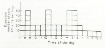
Fig. 3.4 Queueing problem: expected arrival pattern
The next obvious question is how we obtain the 'random numbers' which decide whether 1, 2, or 3 cars arrive. We could use a die, calling 1 and 2 on the die 1 car, 3 and 4 on the die 2 cars, and 5 and 6 on the die 3 cars. If the die is fair, each number has an equal chance of occurring - 1 in 3 throws will give 1 car, and so on.
Any fair chance occurrence can be used this way; before computers were common, people often used specially prepared tables of random numbers or even pages of telephone directories. (Some of the digits in telephone numbers are random once the names are listed alphabetically.)
With computers, the task is generally made easier. As mentioned earlier in the chapter, the computer generates pseudo-random numbers, usually six-digit ones. It is then easy to take, say, the first two digits of each number which will be from 00 to 99 inclusive, of 100 numbers. One-third of the numbers can be allocated to each random event, 00-32 meaning 1 car, 33-66 2 cars, and 67-99 3 cars. (The slight difficulty of 100 not dividing exactly by 3 can be overcome by using only 99 of the numbers or assigning the extra chance to the 'average' as we have done in this case.)
In our example, we use this simple method: for the 'normal' 8 hours of the working day, we assign 1, 2, or 3 cars per 6-minute period, 0, 1, or 2 for the 'slack' period, and 4, 5 or 6 for the high demand hours. In a 'real' simulation, we would be very careful to make sure that the 'spread' we had chosen was realistic, and we might easily choose to make the 5 possibilities 3, 4, 5, 6, or 7 in the high demand hours.
Thus we can use a computer or any other random number source to solve the problem of 'randomizing' the number of arrivals.
Losing customers
How can we decide if customers will be lost by their having to queue? We could observe actual queues and see when customers left. We might find that it is related to the queue size, time of day, or type of car. Whatever we found out could be incorporated into the model, although 'types of car' would require more research and a more complex simulation.
Table 3.6. An algorithm: verbal version
| To the operator of the simulation: | |
|---|---|
| Check how many cars are in the queue. | |
| If there are more than the number of pumps in use | |
| then assume the excess cars will leave the queue. |
We might decide that customers leave the queue when there is already a car waiting and one being served at each pump. If we define the queue as the number of cars waiting (not being served), we can record how customers decide when to leave the queue in two ways, verbally and in the form of a flowchart. In both cases, we call the sequence of decisions an algorithm. The verbal version of the algorithm is given in Table 3.6. We could represent the same algorithm by the flowchart in Figure 3.5.
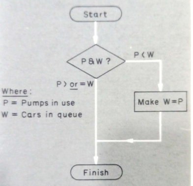
Fig. 3.5 An algorithm: flowchart version
Apart from learning some new 'language' (the shape of the different kinds of boxes, lozenges for start and finish, diamonds for questions, rectangles for operations on variables), one method of re- cording is very like the other and makes clear what condition causes customers to leave the queue. The verbal version tells us that excess customers leave the queue; the flowchart says that if the queue were greater, it would become the same as the number of pumps.
The main advantage of the verbal version is that it is the obvious way to communicate with other individuals: it does not need a new language. The flowchart's advantage is when we wish to use a computer to run the simulation rather than an employee.
Is the simulation realistic?
We can answer the question of whether the simulation is realistic in three ways; by checking the parameters, comparing results, and by repeated simulation.
We can check the parameters used in the simulation by checking on garages in similar situations. Do we have the right number of vehicles at particular times of day, and does the rectangular distribution reasonably represent the probability?
We can also compare the simulation results with the actual results of a garage. Here we are testing whether the simulation, with the same conditions specified in a real situation, reproduces the same overall results as the real garage.
The third method of ensuring accuracy is to run the simulation many times to ensure we do not get freak results. This is where we need computers, and the whole simulation has to be reduced to a flowchart and a computer program. Using the computer is the only cheap and reliable way of running a simulation several hundred times! Table 3.7 and Figures 3.6 and 3.7 show the successive stages of the verbal algorithm, flowchart, and computer program for this particular simulation.
Table 3.7. Garage simulation: verbal algorithm.
|
|---|
|
| Check how many cars are already queuing |
| Pick an appropriate random number of arrivals according to the time of day |
| Add the arrivals to the queue |
| Decide how many cannot be served |
| Decide how many will decide to leave the queue |
| Go to the next period. |
|
| How many cars have been served? |
| How many customers have been lost? |