Five Questions to Help You Prepare For Your University Exam on Keynesian Revolution

Explain How the Keynesian Model Is Applied In a Closed Economy

Use expenditure and income curve (model) to show how unemployment affects expenditure in relation to income. Carefully label the curve showing the changes in expenditure. Finally, explain what a government in a closed economy can do to inject expenditure into an economy.

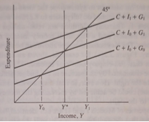
Figure 2.1 The Keynesian 'cross' determination of national income.

The cause of this unemployment is a deficiency of aggregate expenditures. It can be eliminated if the government is prepared to increase its net injection of expenditures into the system. This means that the government should deliberately spend more on the economy than it is raising taxes. In other words, it should run a budget deficit. Previously, of course, the annual budget was simply a way of raising revenue to finance government expenditures. Keynesian economics is an intellectual justification for the use of the budget as the major tool for regulating the level of economic activity.

Model I is often referred to as the income-expenditure system or simply the expenditure system, as in Chapter 1. There can be no doubt at all that the formalisation of the analysis of effective demand failure which it presents was a fundamental breakthrough in economics. Economists of nearly all persuasions have added it to their analytical toolbox and would not question its relevance to the problem it was aimed at, i.e. deep and sustained depression. However, it would be foolish to claim that the apparatus is adequate to analyse other economic problems which have a different origin. For example, what if expenditures exceed full-employment real income at C + l1 + G1? Here it is common to refer to the existence of an inflationary gap (equal to I1 – I0), but inflation itself cannot remove this gap since all variables are in real terms. The model is incomplete. Macroeconomics today is still largely about what has been left out. Keynesians emphasise what was right with the model; Monetarists (and others) emphasise what was omitted.

The expenditure system is certainly not the model of Keynes' General Theory. This is more usually, though perhaps incorrectly, interpreted as being the money-augmented expenditure system or IS-LM model. This itself was introduced by Hicks in 1939, and although Keynes is on record as congratulating Hicks for his attempt to systematise the ideas contained in the General Theory, the model cannot do full justice to Keynes' work. This is Model II of Chapter 1. The only additions are relationships for the demand and supply of money, and a link from money interest rates to investment expenditures. The Keynesian message above can be shown in an exactly analogous way. Figure 2.2(a), for example, shows an equilibrium for the system at less than full-employment real income, Y*. Again, unemployment can be eliminated by an increase in the budget deficit, thus shifting the IS curve to the right. However, in that diagram the same result (with respect to income) could be achieved by increasing the money stock, thereby shifting LM to the right.

Explain the Keynesian Theory of Interest-Rate Determination Showing the Effectiveness of Monetary Policy

The numerical properties of Models I and II are not identical, however. It has already been seen that the multiplier is smaller in II than in I because there is negative feedback from the monetary sector. Higher-income increases the demand for money, which raises interest rates for a given money stock. Keynesians have justified ignoring the monetary sector by the appropriate use of two specific assumptions, though neither is necessary to an understanding of the views of Keynes himself. Indeed, neither is contained in the General Theory. The first of these is that investment is inelastic with respect to the rate of interest (Figure 2.2(b)). If this were true, Model I could tell us all we need to know about the real economy. Money supply affects interest rates but interest rates do not affect any real behaviour. The simple multiplier is now appropriate. The second assumption is that there is a liquidity trap so that the LM curve is horizontal (Figure 2.2(c)). This means that changes in the money stock get 'hoarded" and do not influence interest rates so there are no real effects even if the investment is interest-elastic. This is the famous case of 'pushing on a string'.

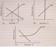
Figure 2.2 The effectiveness of monetary policy in the Keynesian model.

While the latter assumption was used to justify Model I in its early days, British Keynesians increasingly defended their position, in the 1950s and 1960s, by reference to the former. The most influential empirical support for this view of investment behaviour was a survey of thirty-seven businessmen reported by Meade and Andrews (1951), most of whom claimed that the interest rate did not influence their investment decisions. The same survey could be used to sustain the opposite conclusion since a small number of firms admitted that they were affected, which may amount to a significant effect in the aggregate. Until the 1980s it was difficult to establish the existence of an interest rate effect on investment in the United Kingdom, though this may have been due more to the former policy of pegging interest rates than to investment behaviour itself. However, these debates are now of only historical interest, as there now seems no doubt that interest rates do impact investment, as well as other expenditures, including consumption.

There is a special case of Model III which is often called Keynesian. Again it does not appear in Keynes' General Theory but has entered the popular discussion as if it did, following Modigliani (1944). This relies upon the assumption that, while there is no general money illusion, money wages are inflexible in a downward direction.1 If it is assumed that there is an initial equilibrium at full employment, then the aggregate supply curve is vertical above the equilibrium but sloped below the equilibrium, as in Figure 2.3. In effect, the assumption of downward inflexibility of money wages means that there is a money illusion in a downward but not an upward direction. A fall in aggregate demand from AD0 to AD1 produces a fall in prices, but, because money wages do not fall, the real wage rises. At a higher real wage, firms employ less labour and, with a given capital stock, produce less output. So national income falls from Y* to Y1. Employment will remain at this new low level unless there is a reduction in money wages or an increase in aggregate demand. Above the full-employment level of output, an increase in aggregate demand will increase the price level but not the level of real income. We shall see below that the case of real wages being too high is by no means essential for the existence of 'Keynesian' unemployment; the real wage could be below the Walrasian or market-clearing level, and there may still be unemployment in some circumstances. Nevertheless, high real wages may form the basis of what is often referred to as 'Classical' unemployment. Indeed, Keynes himself regarded it as the classical explanation of unemployment.

Moreover, the contention that unemployment which characterises a depression is due to a refusal by labour to accept a reduction of money wages is not clearly supported by the facts. It is not very plausible to assert that unemployment in the United States in 1932 was due either to labour obstinately refusing to accept a reduction of money wages or to its obstinately demanding a real wage beyond what the productivity of the economic machine was capable of furnishing... These facts from experience are a prima facie ground for questioning the adequacy of the classical analysis. (Keynes, 1936, p. 9)

What Keynes clearly did believe, however, was that it is normally money wage rates that are specified in employment contracts so that, at least in the short run, money wages are more sticky than real wages. This was true for changes in either direction.

Now ordinary experience tells us, beyond doubt, that a situation where labour stipulates (within limits) a money wage rather than a real wage, so far from being a mere possibility, is the normal case. (Keynes, 1936, p. 9)

If this were correct, the implications for aggregate supply would be quite straightforward, as we have seen in Chapter 1. The aggregate supply curve, such as that in Figure 2.3, would simply be positively sloped throughout its length. A rise in AD would increase output because higher prices would be associated with lower real wages and increased demand for labour. Higher money wages would increase the labour supply.

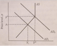
Figure 2.3 Downwardly rigid money wages.

Explain the Reappraisal of Keynes between 1965 And 1977

The simple Keynesian model was dominant in macroeconomics for three decades after the publication of the General Theory. Eventually, its pre-eminence ceased, as more sophisticated Keynesian models emerged, as well as Monetarist and later New Classical competitors. It may be no coincidence that this decline in regard was accompanied by a theoretical reappraisal of 'what Keynes really meant'. This stimulated an upsurge in macroeconomic theory in what was thought to be the tradition of Keynes. However, splitting the Keynesians off from Keynes made them even more exposed to criticism than they were before. After the Reformation came to the Inquisition.

At one level, the reappraisal was a response to the Monetarist criticism that all Keynes' insights could be collapsed into the statement that 'wages are too high', in which case he might as well have written a short letter to The Times, rather than the six books and 384 pages of the General Theory. The reinterpreters asked the question 'how does the economy behave when prices and/or wages are (temporarily) fixed?'. The answer is that there is thoroughgoing disequilibrium; in general, markets will not clear, and agents will be rationed-in particular, they may not be able to sell all their labour and will be unemployed. And this turns out to matter; disequilibrium in one market 'spills over' into others. We can find ourselves in a state of 'Keynesian unemployment' where there is unemployment due to a deficiency of aggregate demand, even if the real wage is below the market-clearing Walrasian level. The prime movers in this reappraisal of Keynes were Robert Clower (1965) and Axel Leijonhufvud (1968), and later Barro and Grossman (1976) and Malinvaud (1977), although the work of Patinkin (1956) led the way.

The Classical (Walrasian) model of a market economy was hypothesised to work by means of an imaginary 'auctioneer'. Transactors entered the market at the beginning of each 'week' with a set of goods and services on offer (supplies) and a set of demands that they would communicate to the auctioneer. There would then be an adjustment process (tatonnement or 'groping'), starting from some initial price vector, such that the prices of goods that were in excess demand would rise and the prices of goods in excess supply would fall. Trade would take place only when prices had been found which cleared the markets, i.e. equilibrium prices. In this way, there could never be an excess supply in equilibrium (e.g. unemployment) because prices would adjust until it was eliminated. This is basically a barter economy since goods would now be exchanged for goods. Every offer of good is simultaneously a demand for another, so Walras' Law (that the sum of excess demands and supplies is zero) must always hold.

One of Clower's contributions was to point out that in an actual monetary economy, Walras' Law need not hold. Suppose an initial price vector exists such that some labour is unemployed. Workers have a supply of labour and a demand for goods. However, the demand for goods cannot be expressed in the market until after workers have received money for their labour. Firms are not going to hire labour until they see the money going down for the goods. It is Catch-22. The actual excess supply of labour is matched by a notional demand for goods, but the effective demand for goods is deficient, so the workers do not get employed and the goods do not get produced.

What is shown here is that the existence of unemployment does not necessarily imply that the real wage is too high but rather that the whole price mechanism is at fault. False signals are being transmitted and there is no tendency for these signals to be quickly corrected. Prices themselves are relatively sticky so it is the quantities of employment and trade which have to suffer, but there is no presumption as to which prices are wrong so the mere reduction of money wages will not guarantee full employment.

However, the reappraisal, while stimulating an exhaustive theoretical investigation of macroeconomics when markets fail to clear, eventually came to a full stop. The essential problem was that although we came to discover what would happen if prices were rigid, we never understood why they were. The informal explanations of why prices might be sticky - for example, the implicit contract approach to labour markets-turned out not to give the right results, as wage stickiness may be quite compatible with market-clearing, given the appropriate environment.

How Has The Keynesian Economics Management Policy Been Beneficial To The Economy?

We now turn to more directly practical matters. It is clear that macroeconomic management in the United Kingdom during the 1950s and 1960s was governed by Keynesian principles. The exchange rate was fixed, so the domestic inflation rate was clearly related to the world rate which was, in turn, very low. Economic policy was largely a tightrope walk with unemployment on one side and balance of payments deficits on the other. If the balance of payments was in crisis, as judged by the official reserves, the economy would be deflated. As a result, unemployment would rise, so reflation would be undertaken as soon as the reserve position seemed satisfactory. This pattern entered common parlance as the 'stop-go' cycle.

The economic instrument which adopted the centre of the stage was undoubtedly the budget, i.e. fiscal policy. Budgets were normally annual events occurring in April, though it became quite commonplace to have 'mini budgets' in July or November. Detailed expenditure plans were generally set in the autumn.2 The experience of the time appeared to be that slightly excessive expansion ('overheating') would be associated with lower unemployment but slightly higher inflation and a deteriorating balance of payments. Overheating would be halted by a budget which raised taxes or reduced government expenditure. Slack would be taken up by the reverse. Monetary policy was not non-existent, but it was largely a residual determined either by the necessity to finance the government borrowing requirement or by the imperatives of the external balance. The money stock was definitely not a target. If anything was a target it was the level of interest rates. In normal times the aim of the Bank of England would be to maintain an 'orderly market' for government debt. Any run on foreign exchange reserves would be countered, however, by a sharp upward rise in Bank Rate, later called Minimum Lending Rate. Monetary policy was thus constrained by the fiscal stance of the Treasury and by the commitment to a fixed exchange rate. It is now more fully realised how these two factors severely delimit the possibilities of independent monetary policy, particularly when international capital is highly mobile. Inconsistencies which arose in the 1960s were increasingly resolved by imposing quantitative ceilings on bank lending. These remained until they were swept away by the reforms known as 'Competition and Credit Control' which were introduced in September 1971.

This concentration on fiscal policy probably explains why (in conjunction with the special assumptions mentioned above) the major forecasting models in the United Kingdom were originally built largely as expenditure systems. Indeed, analysis which focuses on expenditure changes leading through multipliers to income changes is the core of what most economists think of as Keynesian analysis. Later chapters will clarify 'the retreat' from Keynesian policies. However, a few points can be anticipated at this stage.

It is very important not to underestimate the importance of the external environment for an open economy like the United Kingdom. During the 1950s and early 1960s, there was steady growth in world trade and virtually no inflation in world prices. However, during the late 1960s world, inflation began to accelerate, culminating in the commodity price boom and oil price rise in 1973. This has been attributed by some to US policies in financing the Vietnam War and by others to a series of coincidences. If the United Kingdom had retained a fairly restrictive policy during this period the economy would probably have benefited from exported growth. However, the excessive domestic stimulation associated with the policies of the Conservative Chancellor Anthony Barber³, accompanied by currency depreciation, guaranteed that the internal inflationary experience would be worse than that abroad, as indeed the 1967 devaluation had led to a deterioration of domestic inflation. The conventional (Keynesian) macroeconomic theory of the time had incorporated a Phillips curve (see Chapter 7) to explain inflation. This had inflation increasing as the pressure of demand increased. However, in the late 1960s and early 1970s, there were periods of both rising inflation and rising unemployment. As inflation accelerated in the mid-1970s, with no obvious rise in the level of activity, the Monetarist criticisms of Keynesian economics began to gain credibility. Controlling the money supply became a dominant policy goal.

The Keynesian era is often characterised as a period when the authorities were most free to pursue discretionary fiscal policies. Nothing could be further from the truth. While maintaining a fixed exchange rate, the authorities were heavily constrained. Any tendency to over-expansion would rapidly lead to a balance of payments crisis because of reserve losses. Money supply targets and self-imposed borrowing limits were unnecessary because such limits were implicit in the commitment to fix the exchange rate. Thus, it was not that there was no monetary policy in the 1950s and 1960s, it was just that the policy took a different form. Fixing the exchange rate, in fact, implies a far more severe monetary control mechanism than most alternatives.