Questions And Answers That Will Help You Prepare for Your New Keynesians Exam

If your new Keynesian exam is giving you a hard time, go through this blog for help. We have answered some popular questions about this model. These questions and answers will help you prepare better for your Keynesian exam. If you have questions about this blog or our service, email us at support@liveexamhelper.com.

What Is The Position Of New Keynesians On The Fluctuations In Aggregate Demand?

New Keynesians noticed that fluctuations in aggregate demand seem to have real effects, and asked what models of aggregate supply are consistent with this. So this chapter is about some new approaches to aggregate supply, that move away from the Classical view of the world.

At the end of the 1970s, most economists could be classified into one of the camps described in the previous three chapters. The old, unreconstructed- ted Keynesians differed from the Monetarists on empirical issues such as the interest elasticity of money demand and the practical problems associated with interventionist policy; the fundamentalist New Classicists differed profoundly from both, in believing that the analytical roots of the old schools were severely deficient. New Classicists simply did not believe that economic agents could act in the irrational, non-optimizing way that previous generations of economists had allowed. This retreat to fundamental stars struck a deep chord among economists, who prefer to assume that agents always act in their rational interest. The problem for some, however, was that the evidence seemed to conflict with the theory. As we saw in the last chapter, after a promising start, the weight of the formal econometric evidence piled up against the New Classicists.' There was also the informal testimony of everyday experience. Although anecdotes cannot replace proper econometric evidence, it certainly looked like the world had some distinctly non-Classical features. For example:

Wages and prices are usually set for relatively long periods, typically a year in the United Kingdom and often longer in the United States,
Tight government fiscal and monetary policies and other demand shocks appear to have real effects long after they are public knowledge, as in the 1980-81 and 1990-93 recessions in the United Kingdom.
Fluctuations in unemployment do not appear to be voluntarily induced, dominated as they are in the United Kingdom by unemployment spells of very long duration.

Thus, some economists applied US President George Bush's 'duck test' to the economy; if it looks like a duck, walks like a duck, and sounds like a duck, it's a duck. In our case, the 'duck' is a Keynesian model; but at the same time, to satisfy economists' basic requirement, economic agents must be rational maximizers. This rules out the most direct route to Keynesian results, arbitrarily fixing money (or real) wages.

The research agenda of the New Keynesians can be outlined as follows: construct rigorous models of rational maximizing agents where it is optimal to act in such a way that the economy has Keynesian features. This broadly defined agenda has many paths, some of which have already turned out to be dead ends. It is impossible to single out one approach. Nevertheless, several themes have emerged, which we discuss below. We do not attempt to make a comprehensive survey of an extremely diverse and eclectic field; instead, we try to pick out some broad themes and ideas which have emerged in the past few years. A good introduction to the area is given in the two volumes edited by Gregory Mankiw and David Romer (1991), and in the winter 1993 issue of The Journal of Economic Perspectives Vol. 7, No. 1.

How Do Wages Affect The Labor Market?

Long before Keynes, it was appreciated that if wages were insufficiently flexible to clear the labor market, demand shocks would have real effects. Even with rational expectations, as we saw in Chapter 4, the existence of wage contracts lasting longer than one period is sufficient to induce a role for activist macroeconomic policy. What is more, Taylor (1980) showed that where contracts depend on future relative wages, the effects of shocks could last far longer than the duration of the wage contracts. However, the problem with this approach, from the point of view of both the New Classicist and New Keynesian research paradigms, is that lengthy overlapping contracts-wage rigidity itself, in other words - are never derived from theory. Originally, two justifications for these contracts were put forward. First, it was argued that setting contracts is costly. It is unclear to what extent this is true, but it must also be said that economists have an inbuilt resistance to explanations appealing to 'adjustment costs', usually described as ad hoc. The second justification was an appeal to the implicit contract literature of the early 1970s.

The theories of implicit contracts were a microeconomic response to the observation that firms do not usually change their wage scales when demand meets a downturn; wages remain constant while employment and output vary. The ideas were first explored by Azariadis (1975), Baily (1974), and Gordon (1974). The basic insight of the models was that contracts may consist of two elements: an explicit wage, and a (possibly implicit) commitment to employment. The latter effect was hypothesized to work via the employer contracting to lay off workers in bad times at agreed rates. In an uncertain world, a risk-neutral firm would be indifferent between a wide range of wages for good and bad times. For example, if there is an equal chance of good and bad times, ex-ante a firm expects to make the same profits (on average) for a given workforce if 'good' and 'bad' wages were £170 and £10 respectively (average £90), or £100 and £80 (also an average of £90). If workers dislike risk and there is a basic level of unemployment benefits, then workers are best served by constant wages in good and bad states with some random layoffs. Firms are effectively acting as insurance agents for risk-averse workers in this setup. What is more, despite the apparent constancy of the wage, the level of employment that results is the efficient level, that which would hold if wages were free to fluctuate, though it is this last result that gives the game away. The point is that in these models, although wages are indeed constant over the cycle, wages are a veil, in the sense that firms and workers have agreed ex-ante to effectively disregard the fact that ex-post wages may differ from the marginal product. The macroeconomic significance of this is that fixed wage contracts do not necessarily imply the existence of a simple Keynesian aggregate supply relationship. Later refinements (see Grossman and Hart, 1981) incorporating the possibility that firms may cheat by lying about whether they face a good or bad state led the models away from the efficient outcome; but the basic insight endures, that rigid wages over lengthy contracts may not be all they appear to the naive observer. Alternative explanations were required.

Another explanation for wages failing to move to clear the labor market is that they perform more than one function. That is, wages are set not only to attract a supply of workers but also to induce those workers to supply a particular level of effort. As soon as this holds, the wage will in general not be able to clear the market. We have two targets-high effort and full employment - but only one instrument with which to attain them. The explanation for the existence of efficiency wages may lie in one of two possible areas. The first is to do with recruitment and retention. Most firms have at least a little monopsony power concerning the labor market, if only because searching for and moving between jobs is costly. This means that to some extent they must decide on the optimal (efficient) wage to offer. If wages are high, vacancies will be filled more quickly and fewer will quit in any period. Both these phenomena lower costs, and firms will balance a higher wage bill against lower turnover costs. If workers differ in ways hard to measure before hiring, a higher wage will tend to attract applicants who are more productive, on average. Furthermore, the best workers will not leave so readily, as they will be less likely to be poached by higher wage offers elsewhere.

The other area has to do with direct effects on efficiency. This may work via non-economic routes; if a firm pays more than is strictly required by the market, this 'gift' of higher wages may be reciprocated by the employee with loyalty and higher effort (Akerlof, 1982). An alternative story, somewhat less sanguine about human nature and therefore more to the taste of economists, revolves around the idea that firms cannot easily measure effort. (If they could, they would simply demand minimum effort levels from workers and dismiss workers who failed to deliver.) In this case (explored by Shapiro and Stiglitz, 1984) firms set wages high enough to make workers regret being laid off even though workers would find a new job eventually, the wage would be lower and (imperfectly) monitor workers. Some slacking workers will be picked up by the firm's monitoring process and be sacked. The high wage makes this a real threat, and if all firms set high wages, as they must in equilibrium, unemployment results.

These models do offer an explanation for unemployment and rigid wages, but by themselves, they are not the missing Keynesian link we are searching for2. The point is that although wages are higher than the competitive level, they are not 'too high' in the usual sense, based as they are on optimizing behavior. In Chapter 2 we looked at a Keynesian special case, where money wages are fixed at too high a level that is, above - equilibrium. Unemployment results. In that model, expansionary policies raise the price level and therefore reduce real wages, increasing employment and output. In the efficiency wage model, we also have high wages and unemployment; but if prices rise, employers will want to offer proportionally higher wages, as the (real) efficiency wage is indeed efficient for them. Thus efficiency wages, or other stories with similar consequences, do not yet offer a direct connection between aggregate demand and output, which is the characteristic Keynesian proposition. We have part of the jigsaw, but there is a missing piece that connects non-competitive wage setting and output fluctuations. It is to that issue we now turn.

Explain How Fluctuations In Nominal Demand Can Cross Over Into Output Even When Firms Ar Acting Rationally

Both mechanisms revolve around the notion that the advantages of adjusting wages (or prices) to a small demand shock can be extremely small, so that firms may find it more profitable to meet demand by quantity adjustments changing output than by altering prices.

Menu costs, as the name suggests, refers to the costs associated with changing prices (printing new menus, in other words). These costs may be quite small, but as Caplin and Spulber (1987) argued, in the presence of imperfect competition, their existence may have a disproportional effect on aggregate demand - and in fact the costs may be larger than we might expect. Although the physical cost of altering price lists is trivial in many cases, these are not the only considerations. Customer goodwill and loyalty may well be more important factors; higher price lists may encourage existing customers to start searching for better deals elsewhere. In the end this is an empirical question. Carlton (1986) examined detailed data on individual buyers' prices in US manufacturing. He found that although there is evidence that the physical fixed cost of changing prices is low for many buyers, it is also the case that 'The degree of price rigidity in many industries is significant. It is not unusual in some industries for prices to individual buyers to remain unchanged for several years' (Carlton, 1986, p.638). There is also some econometric evidence on the matter. Price (1992a) estimates a model of UK manufacturing price-setting which tests a model with explicit costs of adjustment. The model performs very well, and price-setting occurs with a high degree of persistence, implying relatively large adjustment costs.

The easiest way to see why menu costs matter is in the context of a monopolist. Take the standard textbook model of a monopolist, illustrated in Figure 5.1. Suppose that the firm's demand curve is affected by the aggregate price level P so that the firm's price p is given by :

P = D (Q)P (5.1)

The firm's price p is proportional to the aggregate price level P but is

also affected by other factors summarised in D(Q), where Q is the firm's output. The firm's price and output are negatively related (the demand curve slopes down).

So if q is the real price (p/P) and MC is real marginal costs, we have the situation illustrated in Figure 5.1. At the optimum, output and price are Q* and q* respectively. Now suppose aggregate demand rises, so P increases. If real industry demand is unaffected, the optimal price is unchanged. However, if the nominal industry price is fixed, the real price falls to q, and output rises as demand increases. If so, the firm will necessarily make less profit than before. Nevertheless, because of menu costs, it may not be worthwhile for the firm to raise the price. What is more, the firm will still want to satisfy the higher demand as the extra revenue exceeds the extra cost at this point (MR > MC). This is crucially different from what would happen under perfect competition, where the firm will lose even more if it increases output, as the rise in output will generate less revenue than the extra cost. The key insight is that for small changes in P the profit loss is 'second order" (very small, in other words) as q is still very close to the optimum. Figure 5.2 illustrates the point.

At the optimum, the objective function is horizontal. In terms of calculus, for a maximum we require that dл / Dq = 0. So a small nudge away from equilibrium, say to Q1, will have next to no effect on profits; firms will not change prices. If every firm acts the same way, we find that aggregate demand will affect output - just as in a Keynesian model. Similarly, the same type of argument applies to wages if, as in the efficiency wage model, the firm sets their level. Wage effects are not theoretically necessary, but as Ball and Romer (1990) show, they help to make the resulting effects more plausible from an empirical point of view.

Akerlof and Yellen (1985) had a very similar argument with their concept of 'near rationality'. They argue that in the region of the profit maximisation point wage-setting rules of thumb lead to only second order (i.e. tiny) costs. In a similar manner to menu costs, nominal disturbances are thereby transmitted to output.

The problem is that menu costs do not really work as a mechanism for explaining large changes in aggregate demand. For example, if demand were to rise to the point where q fell to q2 in Figure 5.1, the lost profit might exceed any menu costs. Furthermore, we have only considered a one-off change. A more realistic model would allow for a succession of shocks over time, and allow different firms to be in different positions relative to their optimal price. It turns out that if the direction of shocks is always upward (not too restrictive an assumption given some inflation) then the effect of aggregate demand on output washes out on average (Caplin and Spulber, 1987). On plausible assumptions firms will find it optimal to adjust their price when they hit a particular threshold value for the real price; in expecting the shocks to continue, they raise the price 'too high', above the optimum in the absence of shocks. So on average just as many firms have prices above the optimum as below. An increase in demand pushes some off the top of the distribution their real price hits its floor but simultaneously others are entering at the bottom. On average, the real price remains unchanged.

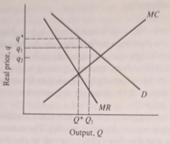
Figure 5.1 Monopoly: real demand and costs.

How Does The Union Objective Function Affect Employment? In Detain Explain How To Calculate The Union Objective Function

An alternative explanation for non-competitive or sticky wages is that insiders those already in employment at firms selfishly disregard "outsiders' the unemployed and those in low jobs - when setting wages. The insiders are often thought of as members of unions. This need not necessarily be the case as most workers have special skills and knowledge that give some bargaining power, but it is convenient to think in terms of a 'union' bargaining with an employer. Certainly, unions are important in Britain, despite the efforts of the Thatcher and Major governments to reduce their power. Unionisation has declined in the United Kingdom so that less than 50 per cent of are now unionised, but this may understate their significance. Table 5.1 shows that in 1984 two-thirds of workers were covered by collective agreements, well above the proportion unionised, although the figure varies widely between industries.

The important issue to grasp is that in the existence of unions, wages and possibly employment are the outcome of a bargaining process, in which neither unions nor firms are likely to get exactly what they want. The first authors to explore this properly were McDonald and Solow (1981), although Leontief (1946) anticipated the fundamental results. The firm's objective is simple: it wants to maximise profit. Things are not so straightforward for the union. Unions may care about a wide range of issues, including personal power and job security for union bosses, political aims, as well as the conventional issues of working conditions and remuneration. However, we focus on the narrowly economic objectives of wages and employment. There can be no doubt that ceteris paribus, unions prefer higher wages to low. Indeed, that may be all they care about; Oswald (1987) offers some evidence for the United Kingdom that is consistent with this view. Yet wages cannot be increased indefinitely without consequence. Eventually, jobs must go. So if unions do consider employment conse- quences, which the balance of the evidence suggests they do, then they must take this into account when bargaining over wages.

We can express this somewhat more formally. The union's objective function ("utility") is given by

V = V (N , W) (5.2)

V is the union's objective function; it is increasing in employment N and real wages W.

A popular version of this general function is that the union maximises the expected utility of its members. The utility that members get will depend on whether they are in or out of work. In work, they receive the wage rate; out of work, they receive unemployment benefits.3 The probability of being employed is simply (1 - u), where u is the proportional unemployment rate.

We can simplify by making a number of assumptions. If union members are risk-neutral then we can treat money returns as equivalent to individual utility. A closed shop makes the identification of unemployment rates and probabilities exact, and assuming that the return to unemployment is zero simplifies the analysis without any loss of generality. Under these circumstances, union utility is given by :

V = (1 - u) MW (5.3)

where M is the union's membership. With the closed shop,

u = (M - N)/M(5.4)

so,

V = NW (5.5)

In other words, unions aim to maximise the wage bill. Some union indifference curves are sketched in Figure 5.3, showing the trade-off between wages and employment.4 A higher wage can compensate for lower employment. Union utility rises as we move to the right or upwards. Although (5.5) guarantees the standard shape, it is natural to assume that the corresponding curves from the general case in (5.2) would also look like this.

Next we consider the firm. If there were no union, firms would simply maximise profits subject to the market wage. Figure 5.4 shows how the demand curve for labour may be derived, using the (possibly unfamiliar) device of isoprofit lines. An isoprofit line shows the combinations of wages and employment yielding particular levels of profit. Maximum profit is at the point where the standard textbook condition holds, namely, that the real wage equals the marginal revenue product. As we move away from this point (which marks the maximum of the isoprofit line) in any direction, with higher or lower employment, the wage must be lower in order to maintain the same level of profits. For any level of employment, lower wages mean higher profits, so the lower the isoprofit line, the higher is profit. Thus the firm will choose the lowest possible curve given the wage, and the tangency points for all the wages map out the (profit- maximising) demand curve. If W* is the market wage, the firm is on l* at N*, point A on the diagram. F marks the zero profit point. This may seem like a long winded way of deriving a downward sloping demand curve, but the derivation has the great advantage of telling us what happens when we are off the demand curve.

We are now in a position to put the firm and union together. In Figure 5.5, the union's preferences are again summarised in the indifference curves, of which V*, V1 and V₂ are shown. If the bargain is restricted to the demand curve, then the best point for the union- the highest attainable utility-is at B. Notice that (in general) this will not be the zero profit point. This point is that which would be chosen in the extreme monopoly union case where the union has all the bargaining power. In general, in this right to manage set-up where the firm and union bargain over the wage but the firm chooses employment, the wage will end up at some intermediate point, such as C. The precise position will depend on relative bargaining power. As union power falls (affected by legislation, for example), the outcome will shift to the right and employment rises.

One problem with this model is that, as Leontief observed in 1946, these bargains are inefficient. Starting from C, both parties can do better by lowering the wage and raising employment. This violates the basic principle of Pareto efficiency, where efficiency is defined (rather weakly) as a situation where no-one can be made better off without making at least one other person worse off. Only points like D, where the isoprofit and union indifference curves are tangential, constitute efficient bargains. The locus of these, ADE, defines the contract curve. On the face of it, this is a remarkable result. Notice that the contract curve lies to the right of the competitive outcome.5 Also notice that if the union becomes more powerful, it will push the bargain up and to the right. So if unions and firms bargain over employment, not only is employment higher (and unemployment lower) than in the competitive case, but an increase in union power will raise employment! In fact, appearances are misleading here, as this is a partial equilibrium model. In general equilibrium, as Layard and Nickell (1990) show, a in union power will lower aggregate employment; but the result still holds for a particular industry.

Whether bargains are efficient or not is an empirical problem. It may be that of imperfect information or high bargaining costs efficient outcomes are unattainable, and this seems to be the case for the United Kingdom: see Layard, Nickell and Jackman (1991) for some evidence on this.

So far there is no particular macroeconomic consequence. Employment may be less than or greater than the competitive outcome. In special cases shifts in demand may leave the real wage unaltered; but this does not by itself lead to aggregate demand affecting output. As before, we need (for example) menu costs.

One basic deficiency of the simple models presented above is that they involve static, one-shot bargains. In reality, unions and firms repeat the bargaining process year after year - a dynamic problem. This leads to several considerations, among which is the growth or decline of union membership. The most dramatic assumptions are, first, that membership is equal to the last period's employment, and, second, that insiders care only about their own expected welfare.

This leads to two apparently contradictory phenomena. First, the insiders want to consider their future probability of being employed. Lower employment now will tend to imply lower employment in future (as the small membership has no incentive to enlarge the pool), and thus a higher probability of being out of the inside group. This gives an incentive to lower wages in bad years-real wage flexibility is higher than in the static case; but there is a second effect working in the opposite direction. If employment does fall, the reduction is likely to persist for a long time. In the extreme, as in Blanchard and Summers (1986), there is pure hysteresis.6 That is, a shock to employment will persist forever; unemployment is permanently higher, The mechanism is that if demand and employment fall in any period, the 'insiders' left in employment are happy to negotiate higher wages reflecting the smaller sized workforce, ignoring those of their previous colleagues who are now outside the bargaining process. If the world is like this, then it becomes very important to avoid adverse demand shocks, as the conse quences may be very severe.

To some extent these results conflict. The insider-outsider models have tended to emphasise the second effect, but it is by no means clear that unions will want to act in this way. However, the hysteresis model based on the insider-outsider approach does offer an explanation of one of the great macroeconomic puzzles; that is, the stubborn refusal of real wages to fall during the two crushingly severe recessions that the United Kingdom has been subjected to since 1979. Indeed, the period since 1979 has seen a combination of very high unemployment (by both historical and interna- tional standards) and high real wage growth (again, on both comparisons).

Table 5.1 Percentage of workers covered by collective agreements in Britain, 1984.

Private
	Manufacturing	Services	Public
Manual	79	53	100
Non-manual	79	40	100

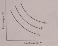
Figure 5.3 Union indifference curves.

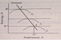
Figure 5.4 Isoprofit lines and the demand for labour.

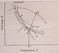
Figure 5.5 Firm and union bargains.

Explain Why Firms Respond To Demand Shocks By Expanding Output And Not Raising Prices

We have already seen how imperfect competition is important in the approaches set out above. Models with menu costs require marginal revenue to exceed marginal cost, which is incompatible with perfect competition, and unions are inherently uncompetitive. Beyond this, the theory of imperfect competition can help to explain directly why firms respond to demand shocks by expanding output, not raising prices, as Weitzman (1982) was among the first to show. This is not enough by itself to generate real effects from changes in aggregate demand, but it helps generate large changes if any exist at all.

One story is that when the demand for output increases, firms lower their profit margins. This could follow if firms and customers have a long-run relationship, encouraging the formation of implicit contracts to keep prices constant. Like the literature examining implicit wage contracts discussed earlier in the chapter, this indicates that rigid nominal prices have no particular macroeconomic consequences, and does not help us in our search for Keynesian mechanisms. Another argument is that competition tends to be procyclical firms price compete more in booms, cutting margins (Rotemberg and Saloner, 1986). More straightforwardly, the elasticity of demand may be procyclical. Standard micro theory tells us that the mark-up of prices over marginal costs is inversely related to this clasticity, so profit margins will fall in booms. More subtly, firms may find it optimal to attract new customers in booms, hoping they will remain attached in the downturn.

Another approach follows from an idea introduced by Sweezy in 1939. This is that firms adjust their prices asymmetrically, leading to a kinked demand curve, as shown in Figure 5.6.

The original rationale for this was based on firms' conjectures about their competitors' behaviour. If a firm expects that other firms will match price cuts, but will hold prices constant when its price rises, then the expected demand curve takes the form in the figure, with a kink at the current price. This creates a 'hole' in the marginal revenue schedule, so that a (small) shift in demand may leave output unaffected. An alternative justification is given by Stiglitz (1979), based on costly customer search. Lower prices will not attract many new customers (who are not looking for new suppliers) but higher prices will put off existing customers. The implication for macro- economics is that if aggregate demand increases, shifting sectoral demands to the right, the price will remain constant (so long as the change is not too large). Thus aggregate demand can have real effects.