How To Tackle Online University Exams On Exchange Rate Models Like A Professional
Discuss in detail at least 3 exchange rate models that can be used the explain the economic history of the UK.
Explain the application of percentage rate of change of exchange rates on monetary growth rates and income growth.
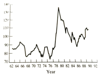
Figure 6.5 UK real exchange rate (series is 'relative normalized unit labour cost') (1985-100). Source: Datastream.
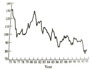
Figure 6.6 UK effective exchange rate 1975-93 (1985-100). Source: Datastream.
a relationship that does hold more or less exactly, so long as appropriate interest rates are chosen and exchange risk is hedged through forward markets. Critical for what follows is the assumption implicit in the dropping of PPP and adoption of interest parity. This is because asset markets adjust quickly and the goods market adjusts slowly. Goods prices are sticky, but exchange rates and interest rates can change rapidly. The model to be discussed is essential due to Dornbusch (1976b).
Consider an IS-LM type portfolio choice between money and bonds. Domestic bonds and money are denominated in domestic currency (obviously) and foreign bonds and money are denominated in foreign currency. Interest parity requires that the expected return on domestic and foreign bonds be equal. If exchange rates can change, the relative return has two elements- the coupon interest yield and the change in the exchange rate.
r=r*+x (6.10)
The domestic interest rate, r, is equal to the foreign rate, r, plus the expected rate of depreciation of the domestic currency. If, for example, the sterling bond interest is 5 percent per period and the equivalent dollar rate is 10 percent, sterling must be expected to appreciate by 5 percent per period. If this were not true it would be expected to be profitable to shift funds to where the return was higher. Notice, though, that the mere fact that one interest rate is higher does not indicate inequality of expected return.
The exchange rate is defined to adjust at some rate from the existing exchange rate e to the equilibrium ē.
X=θ(ē-e)(6.11)
where ē and e are now in logs. Again, we focus on the domestic money market as expressed by the demand for money equation (plus the assumption that supply equals demand).
m-p=αy-λr(6.12)
where variables are in logs, except the interest rate, r. (This is the same as (6.7) if K = exp [-λr].) he foreign economy can be assumed to be 'large' relative to the home economy. This enables us to take the foreign interest rate as exogenously fixed. Substitute (6.11) into (6.10) for x and then substitute this combined expression into (6.12) for r. This gives
m-p= αy- λr*-λθ(ē- e)(6.13)
This is nothing more than the domestic money market-clearing condition when interest parity is imposed as an extra constraint. Notice that in full equilibrium e will equal è, so equilibrium prices will be:
P=m= αy+ λr*(6.14)
This enables us to simplify (6.13) by replacing m- αy+ λr* Rearranging as an expression for the exchange rate gives:
e= ē-(1/ λθ)(p-p)(6.15)
This says that the exchange rate will deviate from the long-run level if the price level deviates from its long-run level. This may not seem p interesting, but in reality, it says a great deal about the behavior of exchange rates.
Consider Figure 6.7 which plots two relationships between the price level and the exchange rate. The positive sloped (45°) line labeled p=e is equation (6.6). This is determined by purchasing power parity. It is drawn on the assumption that units are chosen so that p* is unity.
The negative relation between p and e is given by equation (6.15) for given values of exogenous variables (so given values of è and p). It reflects domestic money market clearing in conjunction with interest parity.
Start at A in full equilibrium and let there be a once-and-for-all rise in the domestic money stock. Let us presume that the domestic economy is at full employment so that income effects can be neglected (a vertical IS curve or a classical aggregate supply curve will do just as well). From (6.14) and (6.6)it should be obvious that in full equilibrium both p and e will rise in proportion to the increase in m. (Recall that e is the domestic currency price of one unit of foreign exchange, so a rise in e is a devaluation of the domestic currency.) This means that the new money market-clearing condition will pass through a point like B which is northeast of A.
However, the economy will only jump straight to B if prices and
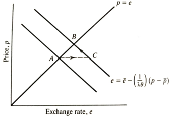
Figure 6.7 Overshooting model of the exchange rate.
exchange rates are perfectly flexible. In that case, the excess money stock would be immediately eliminated by higher prices and the real money stock would be unchanged. It is more realistic to believe that the exchange rate can adjust rapidly, but that goods prices (and money wages) are relatively sticky. As a result, the adjustment pressure will be reflected first in the exchange rate. It will jump up to C and then gradually fall to B as prices adjust over time. This reflects the 'overshooting' of the exchange rate since the initial devaluation is greater than that ultimately required. Further comment on this overshooting is required since it is fully consistent with rational expectation formation.
What happens after a money supply increase if the price level does not immediately adjust? If the domestic output is constrained not to rise, the pressure must be reflected in the domestic interest rate. It will fall. This means that the interest parity condition (6.10) is violated. Since r" is fixed, only x can now change to restore equality. The value of r has fallen, so x must be negative if the domestic and foreign bonds are to have the same expected return. A negative x means an expected appreciation of the home currency. Long-run equilibrium requires a depreciation when compared to the initial point. These can only be reconciled if e immediately depreciates to a point from which it can be expected to appreciate during the adjustment of prices to the long-run equilibrium. This appreciation is just sufficient to compensate for the lower domestic interest rate. Hence, when the money stock increases the exchange rate depreciates too far and subsequently appreciates. This is what is meant by overshooting.
Notice that overshooting depends only on the price level and is relatively sticky. There is no requirement for absolute fixity. The analysis will be more complex in reality to the extent that real income changes. It should be expected to change because at a point like C in Figure 6.7 (indeed, any point off p= e), PPP does not hold so there will be expenditure shifts in favor of the economy with lower prices. In the case of domestic monetary expansion, the exchange rate depreciates too far so domestic goods become relatively cheap (temporarily). With a tightening of domestic monetary policy, the home currency over-appreciates, and domestic goods become relatively expensive.
The exchange rate overshooting model was widely used to explain the over-appreciation of sterling in 1979-81 (Figure Buiter Miller (1981a), for example, argued that the tight monetary policies of the Thatcher Government were responsible. However, they later (Buiter and Miller, 1981b) had to admit that the interest rate evidence was not consistent with overshooting caused by tight monetary policy. An alternative explanation (or perhaps a complementary one) places emphasis on North Sea oil. Britain was becoming a net exporter of oil at this time and the oil price doubled in 1979 (see Chrystal, 1984). The explanation of these events remains controversial, though the idea of overshooting is not widely accepted.
Besides explaining specific episodes of exchange rate misalignment, this analysis also explains why exchange rates in general have been so volatile. The system is recurrently being hit by disturbances or policy changes. If goods prices are sticky, the adjustment will be reflected in the exchange rate which can easily change from minute to minute. Thus, exchange r should be expected to bounce about in response to 'news' in a way that is not possible in other markets. At the outset of floating many commentators argued that fluctuations would be reduced as the system settled down. This has not happened. Even (or perhaps, especially) in a model where actors hold rational expectations, there can be exchange rate overshooting se as goods prices are relatively sticky in comparison to exchange rates.
What are some of the major extensions of the Dornbusch model?
Major extensions to the Dornbusch model involved the incorporation of fiscal policy effects and the modeling of full asset equilibrium. Fiscal policy effects are hard to simplify because there are many different ways in which fiscal policy can be implemented and most of these have real effects, even in full long-run equilibrium. However, the general result that a fiscal policy stimulus leads to exchange rate appreciation (identical to Mundell's floating case) will be illustrated below.
Asset equilibrium is important in overshooting models because the transition to full equilibrium involves current account deficits and sur- pluses. A current account deficit necessarily involves an economy running down its net foreign assets (or increasing its net foreign debt). A current account surplus involves the acquisition of foreign assets.
An unexpected monetary expansion at home causes a sequence of events that can be traced using a model developed by Branson and Buiter (1983). For a simplified exposition of it see Chrystal (1989). Figure 6.8 plots the exchange rate on the vertical axis and holdings of foreign assets (by the home economy) on the horizontal axis.
The economy starts at A. The expansion of the money supply leads to an immediate depreciation of the home currency and a rise in e. If rational expectations formation is dominant, the economy jumps to a point like 8 which is on the new rational expectations consistent path (see Begg, 1982 pp. 31-41). The exchange rate depreciation is caused by incipient capital outflows and it also causes a current account surplus to develop. While the current account surplus persists, the economy is accumulating foreign assets, so it starts to move from B to D. Simultaneously there is a rise in domestic prices, not shown in this diagram. When the economy reaches D,
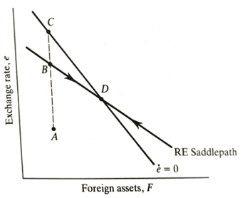
Figure 6.8 Monetary expansion.
the full adjustment has taken place, the current account is back in balance and there are no net capital flows. The domestic price level has fully adjusted to the new higher money supply. However, the economy has a permanent increase in foreign assets.
If the actors in the system had static, instead of rational, expectations, the adjustment process would be similar except that the initial jump would be to C instead of B. This requires a greater initial overshoot of the exchange rate. The reason for this difference is that rational actors know that the exchange rate is going to appreciate from B to D and hence they are prepared to hold more money balances than otherwise - they anticipate the appreciation. Those with static expectations, in contrast, think that the exchange rate is going to stay wherever it happens to be so they choose to hold lower money balances after the initial shock. In other words, those with static expectations dump more domestic money and hence drive the exchange rate down further.
The case of a fiscal policy expansion (see Figure 6.9) is more or less the reverse of the one we have just been through-though recall the proviso that fiscal policy can take many different forms. The economy starts at A. The government borrowing associated with a fiscal expansion puts upward pressure on domestic interest rates. This attracts capital inflows and appreciates the exchange rate. The current account goes into deficit. Under rational expectations, the exchange rate initially jumps to B. It then depreciates back to D while the economy is losing foreign assets. Under static expectations, the jump appreciation is greater initially, than under rational expectations, because the subsequent depreciation is not anticipated. Full equilibrium is restored in both cases at D, where the current account deficit has been eliminated and the country has lost foreign assets.
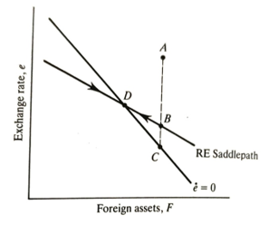
Figure 6.9 Fiscal expansion
Empirical exchange rate models
An enormous amount of empirical work has been undertaken since the late 1970s to test models of exchange rate determination. Initially, the exercise seemed fruitful. Models such as Frankel's (1979) seemed to do well in fitting simple models to the data. However, in the early 1980s, these models broke down comprehensively (for a survey of much of the 1980 literature see MacDonald (1988)). Likely reasons for this failure were the dominance of real shocks such as North Sea oil and the US fiscal deficit Also there was a clear breakdown in traditional monetary relationships in several major countries due to financial innovation. Since exchange rate models were built on demand-for-money equations it was hardly surprising that they would break down too. The key financial innovation in this Context has been the payment of interest on current accounts. Chrystal and MacDonald (1993) provide some evidence that suggests that the simple monetary model may be rescued if 'Divisia' monetary aggregates are used stead of the official simple sum measures of the money supply.
Exchange rate modelers received another blow from Meese and Roge 983). They compared the out-of-sample forecasting performance of a wide range of alternative models. The best one-period ahead forecast was achieved from a model which says that the exchange rate next period is way to the exchange rate this period plus a white noise random error. This casting rule outperforms all economic models and time series forecast techniques. The exchange rate, it seems, is a 'random walk'. The failure of economic models to out forecast a random walk does not necessarily imply that the economy is worthless. Rather it suggests that the foreign exchange market is very efficient (see Levich (1989) for a discussion of efficiency). Efficiency implies that, even if some known economic model were at work in determining the exchange rate, all information relevant to that price (including history and what is predictable about the future) has already been taken into account in setting today's exchange rate. The only thing that can move the exchange rate is 'news- something that was not expected yesterday. News by definition is random. Predicted events that happen are not news in this sense.
In short, exchange rate models should be seen as something which can be tested against historical data and which will inform our understanding of the forces determining exchange rates. However, they do not provide a tool that can forecast future exchange rate changes in anything like a reliable way. The simple message for businesses potentially affected by exchange rate changes is to hedge exchange risk wherever possible and heavily discount econometric forecasts of exchange rate changes. The actual outcome will be dominated by events yet to happen.