Tips for Taking Online Final Balance of Payments and Exchange Rates Exams

Master the skills of taking online final balance of payments and exchange rates exams like a professional. We have prepared a couple of questions with answers based on popular topics and concepts of this subject. You can use these questions for your revision and sharpen your knowledge.

Discuss the analytic approaches to balance payments and exchange rates. Base your answer on the macroeconomic policy in the United Kingdom.

This chapter is concerned with analytic approaches to the balance of payments and also to the exchange rate. The dominant constraint on macroeconomic policy in the United Kingdom during the 1950s and 1960s was perceived to be the balance of payments. The nature of this constraint changed in the early 1970s as a result of major industrial countries adopting floating exchange rates. The sterling exchange rate was floating from June 1972 until October 1990. Then the United Kingdom joined the Exchange Rate Mechanism of the European Monetary System, though it was forced to leave in September 1992. (The issue of regime choice is discussed in Chapter 9.)

The importance which should be attached to balance of payments questions cannot be detached from the regime within which the country is operating. So it is important to remember that institutional changes may seriously affect how these problems are viewed. For example, there is a possibility that the European Community will adopt a single currency by the end of this century. In this event, if the United Kingdom were a member of this currency area, the balance of payments of the United Kingdom would cease to be of great significance - just as the balance of payments of Yorkshire or Devon has had little policy significance in the past (see Chrystal and Wood, 1988).

Explain how the Keynesian or structural approach works.

The Keynesian approach to the balance of payments is based upon an analysis of the balance of trade. In its simplest form, it relies on a single import function and a single export function such as equations (1.3) and (1.4). If we specify the import function so that imports are proportional to income as in equation (1.3).

P=dy

While exports, Xo, remain exogenously determined, then the balance of payments can be analyzed simply in the context of Figure 6.1. Since exports are constant and imports rise with national income, the balance of payments gets steadily worse as national income rises. Beyond a national income of Y, the balance of payments is in deficit.

While this model is a gross over-simplification, it represents a view of the economy which was widely held and which would appear to have been justified by the UK experience. Any tendency for over-expansion in the UK economy produced a balance of payments problems. The experience of the Stop Go cycle in the United Kingdom throughout the 1950s and 1960 seemed to confirm the story that domestic expansion increased imports faster than exports, so the balance of payments inevitably deteriorated. As a result, the expansion had to be reversed. One curiosity, however, to which we shall return, is why it is that this pattern did not seem to apply to other countries. How was it that countries like West Germany and Japan had sustained and rapid economic growth without running into a balance of payments problems? Indeed, Japan has recently had exactly the opposite problem - its economic success was associated with an almost perpetual balance of payments surplus.

Most empirical Keynesian models of the balance of payments, such as those used for forecasting, would, of course, have been more complex than that above. Exports and imports would typically be broken down into several different categories and there would be a term to capture relative price effects. The form of the equation would, however, be similar for each category. Exports depend upon foreign demand and relative prices, and

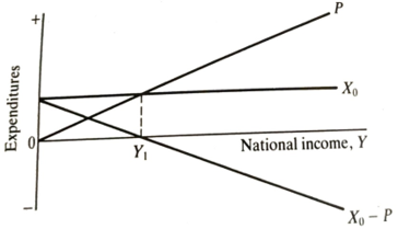
Figure 6.1 Keynesian view of the balance of payments.

imports depend upon domestic demand and relative prices. The overall balance of payments forecast would be obtained by combining all of these import and export categories which had been forecast separately. These Categories normally represent different industrial sectors. Hence, of is a ‘structural’ approach.

Many operational models of the balance of payments had similar thought properties to the aggregate expenditure model above. An expansion of domestic aggregate demand worsens the balance of payments and the addition of a relative price effect can only serve to reinforce this. However, the structural approach to the balance of payments does allow a bias to develop in attributing blame for the balance of payments problems. Since the core of the balance of payments is the real trade account, failure here must be due to inadequate' export performance, these inadequacies being attributable to inefficient domestic industries (perhaps due to under-investment or excessive wage settlements) which are 'uncompetitive. An alternative approach points the finger directly at government macro-economic policy as the source of the problem. This is the monetary approach which is discussed below.

Explain how the Mundell's model rectifies the major inadequacy of the Keynesian approach

One major inadequacy of the Keynesian approach to the balance of payments is that it focuses entirely on the current account. Systematic interactions between the capital account and the domestic economy are thereby completely ignored. A simple rectification of this omission, in the IS-LM framework, was proposed by Mundell (1968). This treatment still provides the basis of many textbook models of the balance of payments. Ignoring capital flows was, perhaps, excusable in the 1950s since there was no general convertibility of major currencies and, as a result, private capital flows were of minimal significance. However, by 1971 financial capital movements were potentially so large that many observers attributed the breakdown of the fixed exchange rate system to their very size and volatility. The liberalization of capital controls continued to such a degree in the 1970s and 1980s that it is common to talk about the 'globalization’ of finance.

The Mundell model is achieved by adding to Model II of the relationship between net capital flows and the domestic interest rate:

K = f(r) (6.2)

Net capital flows depend upon the interest rate.

Capital flows should not be thought of as sales of machines to foreigners, rather they are net sales to foreigners of domestic bonds. There is a problem in drawing the line between the current and capital accounts. In this c 'capital' includes only financial assets. Assuming foreign interest rates to be fixed exogenously, as the domestic rate rises foreigners will b more domestic bonds so the capital account of the balance of payments improves. In effect, foreigners are lending more to the domestic economy Initially, we assume imperfect capital mobility so that a rise in dome interest rates leads to a finite increase in capital flow. The implications f perfect capital mobility follow later.

The overall balance of payments is the current account plus the capital account. The current account gets worse as national income rises just as in the Keynesian model. Thus, if the balance of payments equilibrium is to be maintained (at zero overall) as national income rises, the domestic rate of interest must also rise so that the improved capital account compensates for the worsening current account. In other words, the locus of zero overall balance of payments positions will be a positive relationship between national income and the interest rate, like BB in Figure 6.2.

Equilibrium for the system as a whole requires that all three lines BB. LM and IS should intersect at the same point. Consider the policy choices in the initial situation depicted in Figure 6.2. The IS and LM curves intersect at A where there is full employment. However, this is not a point of balance of payments equilibrium, since A is to the right of the BB curve. There is a balance of payments deficit at A equal to the horizontal distance between A and BB multiplied by the marginal propensity to import. It is open to the authorities to correct the deficit by appropriate use of monetary and fiscal policy, but it is not obvious which to use.

A fiscal deflation would move the economy to point C, whereas a contraction of the money supply would move it to point B. Mundell suggests that the best response is to react with monetary policy to the

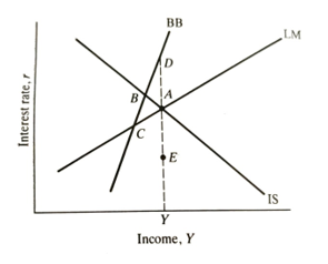
Figure 6.2 The Mundell model.

balance of payments and fiscal policy to output (and thus to unemployment). Consider the contrary. we react to the balance of payments deficit by shifting IS down until it passes through C. This has corrected the balance of payments but caused unemployment. An increase in the money supply now designed to eliminate unemployment would shift the LM curve down to the right. The economy would then be at a point like E where the balance of payments deficit is worse than it was originally. If, however, starting from 4 we change the money supply in response to a balance of payments deficit and fiscal policy in response to unemployment, the economy would converge on point D at which there is full employment and balance of payments equilibrium. This is the reason for Mundell's assignment of monetary policy to the balance of payments and fiscal policy to output and employment.

An alternative version of the Mundell model gives an even better insight into the interaction between policy and external balance when capital is perfectly mobile. This version involves drawing the BB line as horizontal- see Figure 6.3. The interpretation of this is that interest rates are set in world financial markets. Minor deviations of the domestic from foreign rates set up massive inflows or outflows. The domestic economy is effectively a price-taker in the market for bonds. Let us consider how monetary and fiscal policy work under fixed and floating exchange rates.

Consider first fixed exchange rates. An increase in the money supply leads the LM curve to shift right (LM, to LM,). This puts downward pressure on domestic interest rates but as soon as they start to fall there is a capital outflow. This leads to the selling of the home currency in the foreign exchange market. To stop the exchange rate from falling the central bank

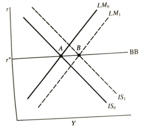
Figure 6.3 Effects of monetary and fiscal policies with perfect capital mobility.

has to buy it back (because they are pegging the exchange rate). This purchase of the home currency reduces the money supply until M return to the original position. Hence a monetary expansion under fixed exchange rates has had no real effect. The monetary expansion has to be reversed to maintain the value of the currency.

A fiscal expansion by contrast shifts the IS curve to the right. With a given money supply, this puts upward pressure on domestic interest rates and, thereby, causes capital inflows. The central bank has to sell domestic currency to stop the exchange rate rising. This increases the domestic money supply, so the economy goes from A to B. Hence, fiscal policy does succeed in generating an expansion where monetary policy failed.

Under floating exchange rates the outcome is reversed. A monetary expansion leads to capital outflows which now cause a depreciation of the exchange rate. The exchange rate depreciation stimulates export demand which shifts the IS curve to the right, so the economy moves from A to B. In contrast, a fiscal expansion leads to upward pressure on interest rates. This causes capital inflows and an exchange rate appreciation. The exchange rate appreciation leads to a fall in export demand which shifts the IS curve back to its original position. In effect, the increased budget deficit is exactly offset by a current account deficit (equal to the capital account surplus). See Chrystal (1989) for a more detailed exposition of this analysis.

In short, monetary policy is redundant under fixed exchange rates (fixing the exchange rate is a monetary policy) but useful under floating rates. The reverse is true for fiscal policy. In this context, it is easy to explain the active role of fiscal policy in the 1950s and 1960s, while monetary policy became more important in the 1970s and 1980s.