10 Thought-Provoking Questions That Each Student Needs To Sharpen Their Skills on Simple Maximizing Models of the Firm

For academic success, you need a proper understanding of basic concepts related to the firm's models. We have outlined some questions that should summarize this topic and provided relevant answers to each of them. Moreover, we also offer exam help services for simple maximizing models of the firm. You can contact us any time.

Basic Concepts Involved In Simple Maximizing Models of the Firm

As we have seen earlier, the most common managerial models involve 'maximizing subject to constraints'. If we model the firm as a whole, we have to decide what it is that the firm is trying to maximize. The most obvious answer is 'profit', and the main concern is the 'marginalist' or neoclassical theory of the firm, which assumes that firms attempt to maximize their profits. An alternative is sales volume or turnover maximization, each of which can be considered, as we do here, as variations of the marginalist model. As most of the models we shall consider have arisen due to dissatisfaction with the marginalist model, it provides an excellent introduction to modelling the firm.

The Marginalist Model

Basic assumptions

Any model of the firm as a whole has to concern itself with seven areas of assumption, which we shall now consider.

What Is Marginalism, And What Does It Assume About Its Relationship To Models Of The Firm?

Marginalism deals with demand conditions by assuming that they can all be summed up in a demand curve or demand function. Specifically, marginalist theory sees firms as either price-takers faced with a market price that they cannot affect or price-makers with a negatively sloped demand curve for their product.

The input supply conditions assumed are that inputs are freely available at known prices. The demand for them by the firm does not affect their price per unit, and there are no constraints on availability.

Marginalism assumes that the decision-maker is the firm's owner, so his objective is to maximize profit. Entry to, or exit from, a particular industry deciding to start or stop production of a particular product, is assumed to be related to the rate of profit. A particular level, called normal profit, is assumed to be necessary to persuade the firm to stay in the industry. If the firm gets less, it will leave: if it gets more than normal profit, this may attract other firms into the industry. Similarly, a firm will move into industries where it sees more than normal profit.

Marginalism assumes that the firm knows about its supply and demand environment with certainty. The firm knows everything it needs to know to make rational, maximizing decisions.

Lastly, the marginalist Theory of the Firm' assumes that the firm can take decisions without looking at what other firms are doing. The result of a pricing decision, for instance, will be summed up in the demand curve. Similarly, the firm's costs will not be affected by the actions of other firms. How marginalism deals with situations where firms have to anticipate reactions is not discussed but is dealt with under strategic interdependence.

What Is The Relationship Between Marginal Cost And Marginal Revenue?

The essence of marginalism is the association of marginal changes with maximization. Marginal cost is the additional cost when the firm changes some aspect of its operations. The marginal revenue of the same change is the addition to revenue. Thus marginalism proposes a simple rule for increasing profit; make a change so long as the marginal revenue is greater than the marginal cost. Of course, this is a general rule, so how does it apply to the price-output decision? The answer is that the firm will seek its profit-maximizing output, the output where no change will increase profit. Behind this is the assumption that marginal cost and revenue depend mainly on output rather than anything else. More than this, certain typical relationships between cost and revenue to output can be discovered.

What Are The Marginal Curves Involved In Models of the Firm?

Cost curves

Marginalism assumes that average and marginal production costs will be U-shaped concerning output, as in Figure 5.1.

In the short run, this is almost bound to be true because of diminishing returns, as explained, but in the long run, there may be industries where costs are constant or even keep on declining. However, the relationship between marginal and average costs is an arithmetic one; when average cost is falling, this is because marginal cost is less, and when average cost is rising, this is because marginal cost is higher. They are only equal at an output of 1 unit and the average cost curve's minimum (turning) point. This point is often called the most efficient output as it is the output at which the average cost per unit is lowest and is, in this sense, at least desirable from the point of view of the community. We see later whether the firm will choose to produce this output.

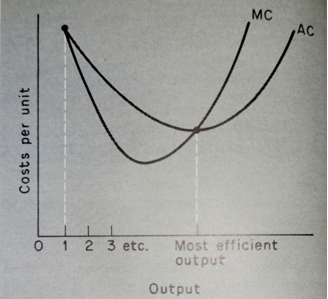
Fig. 5.1 marginalism: typical cost curves

Revenue curves

With revenues, marginalism suggests two different patterns. Firms that are price-takers will have a horizontal average revenue, and their output (assumed to equal sales in this simple model) will not affect the price. This means that each unit sold adds the same revenue as any other unit. Thus the marginal revenue is the same as the average (Figure 5.2).

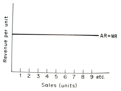
Fig. 5.2 marginalism: revenue for a price-taker

If a firm has to lower its price to sell more, it is called a price-maker. If we take the simplest possible case of a straight-line demand curve, we can see that average and marginal revenue will have the relationship shown in Figure 5.3.

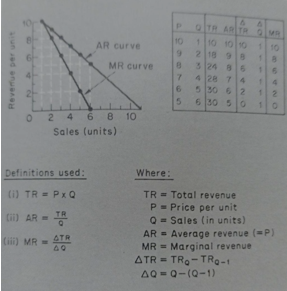
Fig. 5.3 Marginalism: revenue for a price-maker

In our simple example, the quantity (sales) only changes by one unit, so the marginal revenue calculation is very simple: it is simply the change in total revenue. However, when we collect data in real-world situations, we have large differences in the sales and thus must average out the change in revenue by dividing it by the change in sales.

The crucial fact to emerge from the example is that MR declines twice as fast as AR, or to put it another way, that the slope of the MR curve is twice as steep as that of the AR curve. This is true of all sloping demand (AR) curves.

What Is The Overall Output Choice For Price-Takers Involving Both Curves?

We can now combine the cost and revenue curves to determine the profit-maximizing output (and sales) level. First, we consider the case of price-takers. We have assumed that they have some level of profit that they consider 'normal' and necessary to stay in the industry. To simplify the diagrams and the argument, we include this 'normal profit' in the cost curves. So, for instance, when TR = TC (total revenue = total cost), the firm is making enough profit to keep it in the industry. Figure 5.4 shows a possible cost and revenue situation for a price-taker.

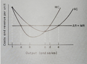
Fig. 5.4 Costs and revenue for price-takers

Which of the five output levels a/b/c/d/e is the one which maximizes profits? First, consider output b, AC AR, so the firm makes a normal profit. Does it pay to increase output? Yes, because for outputs between b and c, an increase in output adds more to revenue than cost (MR>MC). Is c the most profitable output? It is certainly attractive, especially from the point of view of cost, being the lowest possible AC; thus, it is sometimes called the most efficient output. However, outputs between c and d still have MR>MC, so it pays to increase output up to d. If we go beyond d, however, MC>MR, we are reducing profit. So d is the profit-maximizing output.

So profits are maximized when MC MR, but we must also specify what happens to each curve. In our diagram, MC = MR at the output as well. Why is this not another profit-maximizing point? The answer is in the relative positions of the curves. Expanding output at d involves MRMC and so is profitable. So A cannot be a profit-maximizing position. So we need two conditions for profit maximization: MC MR and the slope of MC to be greater than MR's. If you look at output a, the slope of MC is negative, which is less than the slope of MR, which is 0. At d, the MC's slope is greater than MR's.

What is Competition's Effect on Price-Takers?

The effect of competition on price-takers in the previous diagram the firm was in a very pleasant market, being able to choose outputs between B and E and still make at least a normal profit. What if the price were driven down by competition caused by the entry of other firms attracted by the super-normal profit to be made at output d? At what point would the firm wish to leave the industry? It would remain as long as AR was greater than, or equal to, AC. So the price could fall to the level shown in Figure 5.5.

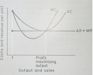
Fig. 5.5 The effect of competition on price-takers

At this point, the firm would have only one possible output, and its maximum profit would be 'normal profit'. One of the attractions of the marginalist model of the firm has always been this result. If the model is realistic, competition will reduce prices until profits are enough to keep firms in the industry, and output will be at its most efficient level.

What Is The Distinction Between This Model And What Happens In The Real World?

In the real world, prices can fall below the level where a particular firm is making a 'normal profit' for two reasons. The first is that the particular firm is not 'efficient' enough, i.e. has higher costs than other firms. The second reason is that firms cannot leave an industry whenever profits fall below normal. Capital equipment may not be suitable for making other products. Thus in industries such as shipbuilding, the firms cannot leave the industry when demand falls off (no one wants to buy shipbuilding yards). So they quote prices that cover their labour, materials, interest, and taxation costs, but not 'normal profit'.

Output choice for price-makers

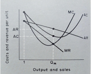
Fig. 5.6 Costs and revenue for price-makers

If we use the relationship of AR and MR from Figure 5.3 and the cost curves from Figure 5.1, we can construct Figure 5.6. Here the firm chooses output Q, where MC = MR, and at this output, AR is higher than AC, and the firm is in the pleasant position of earning more than normal profit. This is the typical marginalist analysis of monopoly, and of course, it can only persist if there are barriers to entry for new firms.

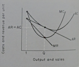
Fig. 5.7 effect of competition on price-makers

If the monopoly is susceptible to competition, the firm may eventually be forced to the position shown in Figure 5.7, where it is just making a normal profit. As in the price-taker model, the AR curve is tangent to the AC curve, but the output is below that necessary for minimum average cost. Thus the marginalist analysis of monopolies and price-makers generally criticizes them as being less 'efficient than price-takers. The main difference between these competitive price-makers and the price-takers is that they produce differentiated products (branded goods) rather than the original. For this reason, competitive price-makers are sometimes called imperfect or monopolistic competitors.

What Are The Achievements Of Marginalism In The Models Of The Firm?

We have now seen the basic features of the marginalist model of the firm as a whole and can make an interim assessment of its value.

The first positive element is its generality. It can analyze competition between producers of un-differentiated products (price-takers), monopolists, and competitive producers of differentiated products (price-makers facing competition). We see its analysis of oligopoly 'competition between the few' - and also, we shall see that those rival models of the firm cannot match its breadth of coverage.

The second positive element is its compatibility with other areas of marginalist theory. Along with other areas not included in this book, they constitute a complete model of microeconomic relationships.

This generality and compatibility lead to the third asset applicability. The marginalist theory of the firm has an impressive list of areas in which it has been applied to forecast the behaviour of firms when faced with problems such as cost increases, taxation changes, and government controls over prices and dividends.

What Are The Criticisms Of Marginalism About Models Of The Firm?

Marginalism has also been widely criticized, and we deal with some of the results of this criticism in this and subsequent. In some sense, the other models of the firm result from gaps in the marginalist model.

First, there is the objection that many firms are not mainly interested in profit but sales (whether in units or value). This 'sales maximization' objective is discussed later.

A second line of criticism has centred on the pricing policies that firms should follow. Research has often shown firms operating other than equating MC and MR!

The assumption about decision-making has been criticized by those who stress the role of professional managers and the effect of different management structures on decision-making.

Strategic interdependence was not incorporated into marginalist theory until comparatively late, and oligopoly has remained an area of weakness.

Lastly, we can argue that firms do not usually build marginalist models of their operations to aid them in decision-making.

Having produced arguments for and against the marginalist model, let us now look at a recent rival, the sales-maximization model.

How is the Sales Maximisation Model a Rival to the Marginalist Model?

An outline

The most detailed outline of the sales (revenue) maximization model is attributable to Baumol (1959). This outline relates to a simple version of the marginal analysis we have already used.

The initial impetus for the theory arose from the observation of American firms that appeared to be attempting mainly to increase their turnover (total revenue) while not neglecting to make enough profit to satisfy shareholders' desire for dividends and provide for future investment. Thus they were maximizing sales subject to a satisfactory rate of profit.

Using our previous analysis, we have to decide whether they were price-takers or price-makers. Assuming, first, price-takers, we could use Figure 5.4 again.

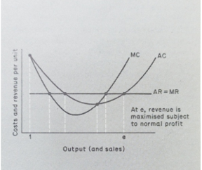
Fig. 5.8 Sales maximization by a price-taker

We have assumed that normal profit will be 'satisfactory' to the firm; if not, we could raise the AC curve by the requisite amount. We can now look at the price-takers position using Figure 5.6 to construct Figure 5.9.

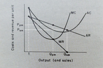
Fig. 5.9 Sales maximization by a price-maker

The price-maker may find that sales (revenue) are at a maximum before above-normal profits are exhausted. At the output, Qsm marginal revenue is 0; thus, outputs beyond Qsm will reduce total revenue, but at this output, AR is still above AC, meaning that the firm is still earning above-normal profit. (Normal profit is included in the AC curve.) The output that a profit-maximizing firm would have chosen is included for comparison, showing that sales maximizers tend to produce more at lower prices. (QPM is less than, and Ppm is higher than PSM-sm). Thus the price-maker seems to be able to make an above-normal profit, as in the case of the profit-maximizing price-maker. However, this depends on the position of the cost curves, as it did in the profit-maximizing case. Thus in Figure 5.9, the firm 'runs out' of revenue it 'runs out' of above-normal profit, but the opposite might occur if costs were higher. Having two criteria (maximum revenue and satisfactory profit) means that one may easily 'bite' in one situation and one in another. So the sales (revenue) maximization model produces the simple decision criterion of profit-maximization; firms will sometimes produce where AC AR and MR=0.

Finally, we can add that under very high costs, or very low prices-sales-maximization may turn out to be the same as profit-maximization. For instance, in Figure 5.5, revenue is maximized at the profit-maximizing output if the firm wishes to earn a normal profit.

Is There Any Significance Of The Sales-Maximisation Model?

Yes, there is. We can identify two major contributions that this model makes, and the first is in introducing realistic assumptions. It attempts to relate the firm's objectives in the model to those found in real-world firms. Managers are keen to increase their salaries and improve the firm's competitive position, and both benefit from higher sales. Moreover, most firms have to consider their shareholders' views and thus maintain satisfactory profits to retain and attract investors. So the model seems more reasonable than one which suggests profits are always maximized regardless of the effect on the firm's size or prospects.

The second contribution is to offer a model of a firm with more than one objective. This, again, is realistic. Firms are not single-minded and have different aims which receive different emphases at different times. However, multiple objectives introduce problems, as we saw in the case of price-makers who were sales maximizers. They needed an 'algorithmic' approach, stopping expanding out- put whenever either of the conditions was about to become unacceptable. This approach is followed up in the 'behavioural theories', where the alternative objectives are said to be satisfied rather than maximized. However, there are also theories in which multiple objectives are jointly maximized, as in Williamson's 'managerial model'. Thus the sales-maximization model leads us naturally into a brief study of 'managerial' and 'behavioural' models.