Spring 2022 Class Test Solution On Demand Forecasting At The University Of Pennsylvania
Exam Question: using relatable theories and surveys, explain how demand forecasting affects models of customer behaviour.
Forecasting without Models
Time-series analysis
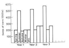
Fig 12.1 A time series graphed
We would immediately notice that there appeared to be a pattern within each year, higher sales in the summer months and that the successive summer peaks were higher. With more investigation, we could put precise figures on the % variations between quarters and the peak demand rate increase. If so, we would have identified two key characteristics of time series, seasonal variation and the trend. If our time series showed such regularity, we would be tempted to expect that it would continue in the same manner next year. Using the trend and seasonal variations already calculated, we could extrapolate the series shown in Figure 12.2.
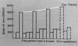
Fig. 12.2 Extrapolation of a time series
Thus we appear to have found a painless forecasting method that does not require any knowledge of the market being investigated. Moreover, the availability of computers means that we do not even have to be able to do the arithmetic! To some extent, this is true; programs (usually called curve-fitting programs) fit a curve to the data fed into the computer and then produce extrapolations of the next few 'months' or 'years. There are also sophisticated programs which look for signs of changes in the pattern and a new branch of mathematics (catastrophe theory) which looks for signs that the pattern will break down altogether (a 'catastrophe').
Looking for regular patterns in economic phenomena is quite sensible; it is how we discover what laws of motion' there are in economic phenomena. At various times people have discovered trade cycles lasting 8-11 years in the nineteenth century, 'stock-cycles' lasting 30-40 months in the twentieth century, and "Kondratieff cycles' of 35-50 years over the last 150 years. Others claim to be able to forecast the behaviour of share prices by looking at the pattern of past prices rather than economic forces. All of these patterns have something to commend them. They are successful in some cases. However, apart from the possible area of catastrophe theory, they do not appear to deal very well with changes in the pattern. To take our simple example of car sales, they would not be able to predict the effect of a sudden increase in oil prices. Extrapolation requires that the information within the time series is enough to explain its behaviour. Many time-series analysis methods are extremely sophisticated but only use the information within the series. They say how things have changed rather than why.
Barometric indicators
Another way of using published information is to look for variables which act as barometers for the variable you are interested in. A barometer measures the changes in pressure before the weather changes. Similarly, some sectors. Of the economy change direction before the economy as a whole. In the US and UK, there are indexes made up of these 'leading indicators', quoted by people wishing to forecast upswings or downswings; Barometric indicators do not forecast. Second-hand car sales often increase before the rest of the US economy turns up. No one suggests a cause-and-effect relationship. The sales figures are quite objective, but they do not cause the thing to be predicted. Thus, we do not have a model; we have a relationship that may be accidental and change. Barometric indicators might work, but like time series analy, we never know when they will fail.
Intention surveys
One of the most obvious ways of forecasting might be to ask people what they are going to de. For instance, many macroeconomic models have investment as an exogenous variable (not determined within the model); thus, we need some forecasts of investment in the next few quarters to forecast other variables. In the UK, there are regular surveys of investment intentions carried out by the CBI (the main employers' organization), which are often used. Commercial market survey organizations also ask householders what consumer durables they intend to purchase over the next a month or a year. These surveys are often reasonably accurate, but their use by firms is sometimes disappointing. The reason is that intentions to invest are reasonably certain; they take time to plan and are difficult to stop once started. The intentions of consumers seldom require much planning and are easy to postpone; moreover, customers are often accurate about their intention to purchase a product but much lew accurate about the firm it will be purchased from. Asking questions about specific products often produces reticence and false answers. Thus intervention surveys, too, have their drawbacks.
Economic Theories
Economists have always assumed that the behaviour of consumers could be predicted by assuming that they tried to obtain as much satisfaction as possible from their limited income. Early theories concentrated on how consumers responded to price changes and how income affected demand for particular products in the twentieth century. We now look at the contribution of these two approaches.
Utility theory and price elasticity
Around 1850, economists began to produce a formal theory of why customers might buy more when prices fell. They assumed that the customer had a fixed income which he spread between products, so 2s to maximize his satisfaction. This satisfaction was termed a utility. For any one product, the utility per unit bought would be less than the more units you had already. If you had a car, the utility from s second car would be less than from the first one etc. If the utility from the last unit consumed was termed the 'marginal utility', we could term the fall in utility from the last unit consumed diminishing marginal utility.
Thus we have reasoned from observations about human beings (the more you have, the less you value additional units) to the stage where we have an explanation for the shape of individuals' demand curves for products. If there is diminishing marginal utility, people will have to be offered lower prices to persuade them to buy more. Thus demand curves will have a negative slope as in our simple demand and supply model. Utility theory is a good example of economic theories; they are often well-accepted facts and seek to show what logically follows from a particular fact. Controversies over utility theory's details have often obscured its main contribution, explaining why individual consumers almost always have negatively sloped demand curves.
We saw that we could express the demand curve in the form of an equation and, if it were a straight line, express the relationship be- tween price and demand by the slope parameter of the linear equation. Economic theory has traditionally assumed the relationship between price. And demand will not be linear; demand curves will be curves. Instead of the relationship being Da-bP, it will be D. ap, as in Figure 12.3.
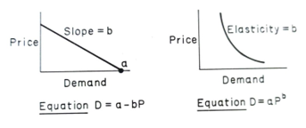
Fig. 12.3 Linear and curved demand curves
Presumably, each of these demand curves will apply in different cases. Some firms or products will have linear and some curved demand curves. Each has its advantages: linear relationships are easier to work with, but curved relationships are easier to explain. The explanation hinges on a mathematical property of 'power functions' (D= aP is a 'power function because P is raised to the power b); when the independent variable P changes by x%, then the dependent variable D changes by the same xe multiplied by b. For example, if b is -2, a rise in the price of 10% will cause demand to fall by 20% [10% x bl. The parameter b is called the price elasticity of demand, defined as 6 changes in demand % change in price. The crucial assumption is that diminishing marginal utility causes curved demand curves and that these curves will have an equation of the form D=aP, and thus once we have found the parameter b, we have an easy way of forecasting the effect of price changes.
Price elasticity: strengths and weaknesses
The great advantage of price elasticity is that it is a simple, easily understood way of forecasting the result of price changes. Moreover, it is answering a great need; firms need to plan output in light of future prices, and governments need to know how consumers will respond to higher prices.
However, like all simple answers to great needs, price elasticity is deceptively simple. It uses the simple model of cause and effect, one independent variable and one dependent variable. Thus it suffers from the usual drawbacks: its true value is difficult to calculate, and even if we have the true value of price elasticity, prices seldom change without other variables changing too. To put this in concrete terms-if, the price of our product went up 15% last year, and demand stayed the same, it does not mean that price elasticity is 0. It probably means that the price rise damped down the 'natural growth of the market. Thus we need to make our model of what affects demand a little more complex.
Indifference analysis and income elasticity
The successor to utility as an explanation of consumer demand was a marginalist version of consumer theory called indifference analysis. Like utility analysis, it starts from a view of human behaviour and sees what this logically entails. This view of human nature sees people as being able to choose amongst combinations of goods. For instance, if people had to choose between food and clothing combinations, they would prefer a set like a to one like b in Figure 12.4.
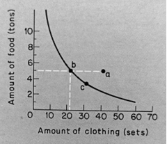
Fig. 12.4 Indifference analysis: the shape of curves
This is because a involves more clothing and no less food than b. It involves two hidden assumptions: that the goods concerned are not 'nuisances', i.e. worth having and that the person concerned is not 'satiated' with either good. However, these seem unexceptionable assumptions to many theorists, and thus they produce the indifference curve going through b and c in Figure 12.4. This joins sets between which the consumer cannot choose. He feels as 'well off at b as he does at c. These curves will have two interesting properties:
- They will have a negative slope; A positive slope would mean not being able to choose between e and a, where a has more of both goods; A horizontal curve would mean not being able to choose between b and a, where a has more clothing: a vertical curve would mean not being able to choose between, say, c and a set with the same amount of clothing and more food.
- They are convex to the origin, as in figure 12.4. As the consumer has less food, he finds it more valuable and requires more clothing if he is to give up a given quantity of food. This property is called the diminishing rate of substitution of one good for another and is the equivalent of the diminishing marginal utility of the utility model.
So far, we have said nothing about money, prices or income and have merely graphed the customer's feelings about two products. We can now go on to add the monetary dimension. We shall bring in money to measure the constraints on our consumer's choices. If we can construct one indifference curve, we can construct others, and the ones to the northeast will represent higher satisfaction levels. Thus the consumer will be trying to get onto the highest indifference curve. What will constrain him? It will be income and the prices of goods. A budget line can represent these as in Figure 12.5. To construct this line, we need to know the consumer's income, clothing and food price. Here we have assumed an income of $6000, clothing priced at $100 per set, and food at $1000 per ton. Thus if the whole income were spent on food, 6 tons could be bought. Alternatively, 60 sets of clothing would take all of the income. Other combinations on the straight line could also be bought. Thus the budget line represents the constraining effect of income given present prices.
We now explore how this analysis can be used to show the effect of price and income changes, as shown in Figure 12.6.
| Y = $6,000 | Y1 = $6,000 |
| Pf=$1000/ton | Y₂ = $8,000 |
| Pc=$100/item | Pf=$1000/ton |
| then $60/item | Pc=$100/item |
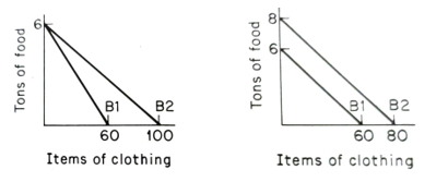
Fig. 12.6 Indifference analysis: price and income changes
We calculate the price elasticity by taking values from the graph, as shown in Figure 12.7.
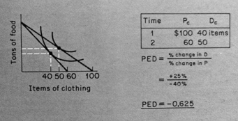
Fig. 12.7 Indifference analysis: price elasticity
Similarly, income elasticity can be calculated in Figure 12.8.
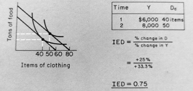
Fig. 12.8 Indifference analysis: income elasticity
Thus we can now think of a more complex model where DaPY and both price and income elasticities could be used for forecasting. This model, with its two independent variables, is often very effective. Still, economists have often had great difficulty persuading other forecasters to extend their models to include price and income. The classic examples in the 1970s were methods of forecasting the demand for fuels such as oil, natural gas and electricity, which relied on a relationship between changes in national income and changes in demand for the fuel. Of course, this implicitly assumes that the price elasticity of demand for the fuel is negligible. The result was that when large price rises did occur, the forecasters were surprised by the demand cutbacks. To take this example a little further, two possible explanations exist for the response to fuel price changes. The simplest is to assume that there is a small price elasticity of fuel demand, which is usually masked by the large income elasticity. Thus the elastic price elasticity is only revealed when incomes stop rising, and prices rise by very large percentages-precisely what happened in the 1970s. (In the case of a particular fuel such as electricity, the price elasticity is only 'revealed' when its price goes up faster than other fuels, natural gas in particular.) But more realistic. It assumes that customers have a zero price elasticity of demand for fuels for prices close to the present price but that for large price changes, it is worth making changes, buying a fuel-efficient car, or changing the fuel for a factory steam-raising plant. The demand curve would look like that of Figure 12.9.
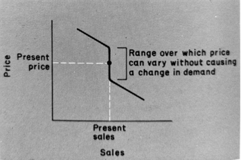
Fig. 12.9 Possible demand curve for fuels
Thus there is a 'threshold."
for price changes beyond which the price elasticity becomes significant. There may also be "thresholds" for income elasticity, and models containing thresholds have been proposed to explain the demand for consumer durables.
Thus we have two distinct contributions from economic theory, a model containing price and income elasticities of the conventional kind and models containing thresholds below which the consumer does not respond to price and income changes. What do other disciplines have to offer to demand to model? We can only sketch some basic outlines, but we now look at behavioural science and marketing for their contribution
Contributions from Behavioural Science
The behavioural sciences, psychology, and sociology have made numerous contributions to our knowledge of how consumers behave. We look at them under two broad headings, motivation research and the use of questionnaires to gather data.
Motivation research with human motivation has produced innumerable studies of the variables which appear to affect behaviour. Many can be used in designing packaging, displays, public relations and advertising. However, they are difficult to incorporate into quantitative models and may be considered as defining effective marketing rather than as variables to be manipulated. Very often, a product can appeal to different customers by directing their attention to different aspects or 'characteristics' that it possesses. Thus there may be no need to trade off one group of customers for another, as is the usual case with market models. So motivation research may offer a relatively cheap way of increasing sales, rather than some more variables to incorporate in a forecasting model.
However, some models need detailed behavioural assumptions that concern customer reactions to individual brands as opposed to the product as a whole and short-run as opposed to long-run reactions. This is similar to the situation with models of the firm: marginalism can deal with industries as a whole and in the long run. In contrast, behavioural theories deal best with individual firms and the short run. An example of a behavioural demand model is the Kappa model, where detailed assumptions were made about why particular children became habitual buyers of one product.
Motivation research also lends credence to theories about perception and reaction thresholds which can be used in forecasting customers' responses to income and price changes. For an insight into the uses of behavioural science in forecasting and marketing, readers are referred to Gabor (1977).
Questionnaires
Questionnaires were pioneered by behavioural scientists as a means of gathering data, and they are one of the main methods used in market research. They can identify customers who will use particular shops or products. People are questioned about their purchases, and their sex, social class and income levels are also noted. It is then possible to correlate the purchase frequency with sex, social class or income, providing valuable information about customers who do and do not buy the product.
There are two main sources of danger in using questionnaires. The first is how the questions are designed and the way they are asked: this point is well-covered in many marketing texts. The second problem lies in interpreting the data. As we have seen above, correlation does not imply causation, raising many problems. Thus questionnaires are a useful source of information, perhaps of testing ideas, but not a source of new forecasting models.
Contributions from Marketing
Marketing tends to be practical rather than theoretical, and we now look at two rather different tools of marketers to see if they can be incorporated into forecasting theories, product life-cycle and test marketing.
The product life-cycle
The essence of this concept is that products go through a life cycle of growth, maturity and decay and those particular marketing policies are appropriate to each stage. Some actions can be taken to prolong the stages, and some companies deliberately shorten the life of products (Other companies may choose to operate in markets where the life- cycle is very short. The extreme, successful examples are companies such as 'Wham-O' in California, which cater for the 'fashionable toy' market.) Like many other useful ideas, the life-cycle hypothesis is difficult to test and thus difficult to quantify for use in forecasting. For more information on how marketers use it, readers are referred to marketing texts.
Test marketing
Test marketing seems to be the obvious way of forecasting product demand. It is the equivalent of the experiment in the engineering field, the chemical engineering pilot plant, and the aircraft production prototype. This new product could be tried out in 'typical' cities, and the results analyzed to see if the product is likely to sell well nationally. Similarly, we could test the reaction of groups of consumers to price changes and thus obtain price elasticities directly. The last process (sometimes called 'consumer clinics) and what is normally called test marketing do have significant drawbacks, as most of their users realize. The basic difficulty is the familiar problem of all social science experiments, namely whether the conditions obtained in the test market will obtain nationally. In particular, we cannot be sure that the long run will show the same pattern as our two or three-week experiments. Customers often respond very differently to introductory offers' than to the usual price. Initially, they may wish to try a product, but a few more weeks of experimenting might tell the observers that the old brand's loyalties would reassert themselves. Another problem with test marketing is a cost against accuracy. Good tests take time and may be very costly to set up and monitor. For instance, if we wish to sell the product at its 'eventual' price under mass production, we will have to sell it below cost for the trial period. The longer the trial, the greater the cost, so firms use short trials with less accurate results.
A related problem with test-marketing and consumer clinics is the so-called 'Hawthorn effect' (first discovered in a protracted series of tests on working conditions) which is that people being experimented on come to enjoy the experience and eventually react favourably to almost any stimulus they are offered. Thus prolonged use of a particular city for test marketing may produce a good reaction to almost any new product.
Therefore direct experiments will probably be more useful for trying out particular ideas than producing quantitative data for forecasting models, and this is how most marketers now use them.
A Synthetic Demand Model
Is it possible to synthesize the ideas to produce a general forecasting model? The short answer is that we cannot produce a general model, but we can produce an approach based on three principles, cost-effectiveness, a priori knowledge and continuous improvement. Cost-effectiveness is easy to explain and entails using the cheapest method of achieving the desired forecast. Thus simple non-model approaches should be used if they are cheaper and do not have obvious drawbacks in the particular situation. Thus we are trading off their lower cost against lower accuracy and the danger of being surprised by events. Similarly, a simple model with only price and income elasticities may be sufficient for many products. Only in some cases will the extra cost of more variables or behavioural assumptions verified by careful surveys be worthwhile.
A priori knowledge is the cornerstone of model-based forecasting methods. We need all the insight into the market that we can get from brand managers, sales associates, economic theory, behavioural science and marketing theory. This enables us to produce a hypothesis which can be tested statistically or by testing marketing Experiments and statistics can test models, but they cannot be their source. As we said before, correlation does not prove causation; the proof has to come from outside the data from a priori knowledge.
The continuous improvement follows from this because any good forecasting model will need continual checking and refinement. The customers will change their tastes, and new products will enter the market. A change of government may change the income distribution or the taxation pattern. As the product is sold, more information will become available, and as it goes through its life-cycle different marketing policies will become appropriate. Thus the forecasting model will need continual review to keep its predictions on target.