13 Questions To Gauge the Understanding of Your Monetarism College Exam Readiness

As a focused student, you try as much as possible to understand the concepts of what is taught in class. You also do well to do more research for a clearer understanding. However, there are thought-provoking questions in monetarism that could make you doubt your readiness for the exam. Our reliable micro-economics exam doers have engaged some of these questions and provided fitting answers. We are a click away if you are looking for professional economics exam help services. Contact us today and get to improve your performance.

Understanding Monetarism through Thought-Provoking Questions and Answers

'Monetarism' was first coined by the late Karl Brunner in 1968. It refers to an approach to macroeconomic policy which gives control of the money supply a central role, particularly in controlling inflation. This approach became important in the United Kingdom in the mid-1970s when, after the abandonment of pegged exchange rates, inflation reached its highest peacetime level since the reign of Henry VIII. The cause of this inflation was widely accepted to have been (mainly) the rapid monetary growth that followed the Competition and Credit Control reforms of 1971.

When Were The Monetary Targets Implemented and Abandoned For The Government?

Monetary targets were an explicit tool of both the Labour Government after 1976 and the Conservative Government (elected in May 1979). However, faith in the Monetarist approach was severely dented in the early 1980s when financial innovation (see Chapter 8) shifted the underlying money demand relationships. Monetary targets were abandoned in 1985, even by a government committed (allegedly) to a Monetarist strategy. That there followed a renewed bout of inflation may be no coincidence. An exchange rate target was adopted in October 1990 when the United Kingdom joined the ERM of the European Monetary System (EMS). However, speculative pressure forced the United Kingdom to leave the system in September 1992. The guiding principles of monetary policy are thus still in doubt.

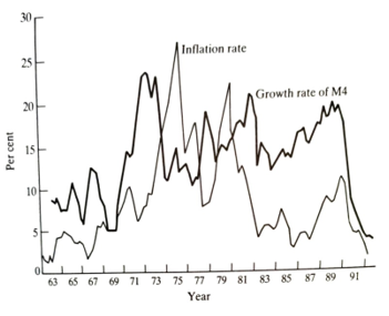
Monetarists are skeptical about the possibility of a successful stabilization policy. There are 'Long and Variable Lags' involved in policy formation and implementation, and there is a good chance that government action to control a cycle will make it worse. The effects of the policy will impact when the condition it was aimed to correct has already changed. Figure 3.1 shows the growth rate of broad money, M4, and the inflation rate from 1963 to 1992.

Figure 3.1 Inflation and the growth rate of M4. Source: DataStream.

Monetarists favor rules versus discretion - whether it should be a money supply rule or an external convertibility rule is more controversial (even among Monetarists). However, the 'correct' approach will vary from country to country.

What Is The Distinction Between The Monetarism Discussed Here And The Political Monetarism?

Confusion should be avoided between the term 'Monetarism' used here and the popular usage which links it to political leaders like Margaret Thatcher and Ronald Reagan. While Mrs. Thatcher claimed to want to use monetary policy to control inflation, her monetary policy was far from what Monetarists recommended (see Chapter 8). Indeed, her government abandoned monetary targeting in 1986. The distinguishing feature of Mrs. Thatcher's ideology was not monetarism but laisser-faire liberalism. She wanted to disengage the government from the economy and, wherever possible free upmarket force. This is discussed further in the last section of this chapter. Let us now look at monetarism in the context of textbook models.

What Textbook Models Best Discuss the Monetarism Theory?

Money in Static Models

Monetarism is first discussed in the context of textbook models; I have no room for a Monetarist interpretation since it has no explicit monetary sector or assets. In Models II and III, the cases identified with monetarism are often called 'Classical' cases.

The orthodox version of the Classical case derives from what can be thought of as a special case of equation (1.9). This special case relates to what is commonly known as 'the quantity theory of money, though in Classical economics, it would be better called "The Monetary Theory of the Price Level.' In modern economics, it is part of the theory of the demand for real money balances. The quantity theory was based on an identity known as the equation of exchange:

MV = pT

Where M is the number of units of money in circulation; V is the number of times per period each unit is used (velocity); p is the average price level per unit transaction; and T is the number of unit transactions per period. This merely says that the value of money paid out in transactions equals the value of goods sold. The theory is achieved by adding the assumption that V and T' are constant, or at least exogenous to the monetary sector. Hence, we have a theory that prices are proportional to the money stock (a gold standard model that was exogenous).

The modern version of the quantity theory is not based on the turnover of money like the equation of exchange but on the average money balances demanded to be held. The primogenitor of the demand for the function is, ironically, known as the Cambridge Equation since it was associated with such famous Cambridge economists as Pigou and Robert- son. The Cambridge Equation says either that individuals hold nominal money balances in proportion to their nominal income or that they hold real money balances in proportion to their real income.

M = kYp (3.2)

M/P=kY (3.3)

Where M is the money stock, Y is income, p is the price level, and k is a constant. By the late 1950s, however, when Friedman tried to provide empirical support in the United States for a relationship similar to (3.3), this equation was no longer part of the apparatus of Cambridge economists. Indeed, it was complete anathema to most of them.

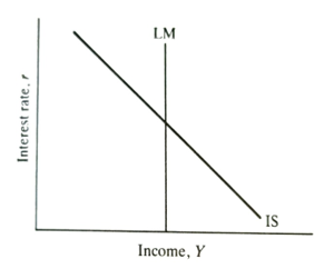
The only differences between (3.3) and equation (1.11) are that income is not presumed to be fixed at its full employment level, and the interest rate is missing here. The implications of this for the IS-LM diagram are straightforward. If we consider the fixed price level case, it is clear in Figure 1.2 that if the demand for money does not depend upon the interest rate, the demand-for-money line is vertical. This means that for each level of the money supply, there is only one income level at which the demand and supply of money will be equal. The implications for the LM curve are shown in Figure 3.2. The LM curve is vertical.

Figure 3.2. LM curve with interest inelastic money demand

The policy implications of this case of the model should be obvious. Monetary policy means changing the money supply, which shifts the LM curve. Fiscal policy shifts the IS curve. If income is the target variable, it is clear that fiscal policy will not affect income, only the interest rate. Monetary policy is the tool needed to control income. It is worth noting that, although textbooks often call this the Classical case, it is far from classical in the fixed price level case. Only at full employment could Figure 3.2 represent the Classical case, and as a result, monetary policy would only affect the price level and not real income.

It must be emphasized immediately that not even extreme Monetarists would likely subscribe to the vertical LM theory today. Although Friedman, in his early empirical work in the United States, Friedman claimed to have estimated a demand-for-money function in which the interest rate was insignificant, the vast bulk of work done since has found the interest rate to be important. So, while this case is of historical interest, it should not be taken seriously as a practical possibility.

An alternative interpretation of the 'Classical' case, which Monetarists may be more likely to subscribe to, can be considered represented by Model IIIB. Here there is a supply side to the economy. Both labor supply and labor demand depend upon the real wage. This means there is no change in aggregate output in response to shifts in aggregate demand. Changes in aggregate demand only affect the price level. This case is illustrated in Figure 1.6, where S is the aggregate supply curve. A shift in aggregate demand from D to D will raise the price level from PO to P, but there will be no change in real income. This is when the price level is proportional to the money stock. An increase in money shifts the LM curve and the aggregate demand curve to the right. Prices rise, as above, restoring the real money supply to its original level - shifting LM back to its original position but with a permanently higher price level.

This is a significant analysis and should be contrasted with the analysis in Model II. However, it should be emphasized that even those who subscribe to this view would regard it as an l case and not an accurate description of the short-run behavior of the economy. We shall see in Chapter 7 how short-run behavior is incorporated into this framework.

In Model II, there seemed to be an important distinction between monetary and fiscal policy. However, in Model III, monetary and fiscal policy can be seen as complementary aspects of aggregate demand policy. Aggregate demand policy is of limited use, especially in Model IIIB, because the real output is not affected in the long run by shifts in demand. Only the price level changes. Thus, even in this simple static model, there would seem to be little mileage to be obtained from making a critical distinction between monetary and fiscal policy. This point is reinforced when it is realized that the possibilities for independent monetary and fiscal policies are severely limited anyway. Deficits have to be financed, and this financing has portfolio effects even if deficits do not lead directly to money supply increases.

To summarize, monetary policy is of no importance in Model I. In Model II, there is a clear difference between monetary and fiscal policy. Whichever is more powerful in controlling national income depends on the shapes of the IS and LM curves. In Model IIIB, the real national output is independent of monetary and fiscal policies in the aggregate. This last case comes closest to the spirit of modern monetarism. However, many aspects of the latter have still to be mentioned, especially about the short-run behavior of the economy.

Indeed, the major distinction between Monetarists and New Classical economics precisely concerns the short-run behavior of the economy. The former would regard aggregate supply as responding to an increase in aggregate demand in the short run, whatever the nature of that demand increase; the latter claim that only unanticipated' changes in demand will have real effects. In the long run, there would be little disagreement.

The Real Balance Effect And The Transmission Mechanism May Result In Modern Monetarism Discrepancies. What Are Some Of These Discrepancies?

The story about how money supply changes are transmitted through the economy is important to understanding modern monetarism. The mechanism built into Models II and III is essentially the link proposed by Keynes, which many would now see as insufficient. This relies upon changes in money stock first, causing portfolio disequilibrium. There is an excess money supply in portfolios and, therefore, excess demand for bonds. This leads to a rise in the price of bonds, equivalent to a fall in interest rate. The fall in interest rate then produces an increase in investment which, through the multiplier effect, influences income. As we have seen, much of the Keynesian disregard for monetary policy arose from the failure to find convincing evidence of a significant interest elasticity of investment expenditure. However, many in the Monetarist camp believe that the link between money and expenditure is much more direct. The direct link is often called the 'real balance effect".

The form of the real balance effect was known as the Pigou Effect. This was usually applied to the behavior of an economy in a depression when the price level was low. The effect arises because the low price level means that the real value of money balances is high. Consumers, in effect, make a capital gain on their money holdings and, as a result, spend more than they otherwise would for a given real income. The Pigou Effect was originally presented as an analytical device that would stabilize the macro-economy since prices would not fall indefinitely.

The real balance effect is more general than the Pigou Effect, though it relates to the same behavioral phenomenon. Anything which causes real money balances (or perhaps real liquid assets) to deviate from their desired level will cause a change in expenditures while the desired level of real balances is out of equilibrium. Thus a rise in the money supply could lead directly to an increase in expenditure. Instead of the excess money balances being reflected entirely as an excess demand for bonds, there would also be an excess demand for goods. The system cannot reduce its holdings of nominal money balances, so the excess real money balances must be eliminated by either price level or real income increases until the nominal money supply is just demanded. Friedman has summarized this as follows:

If individuals were to try to reduce the number of dollars they held, they could not all do so; they would simply be playing a game of musical chairs. In trying to do so, however, they would raise the flow of expenditures and money incomes since each would be trying to spend more than he receives; in the process, adding to someone else's receipts and, reciprocally, finding his own higher than anticipated because of the attempt by still others to spend more than they receive. In the process, prices would tend to rise, reducing the value of cash balances, that is, the number of goods and services that the cash balances will buy.

While individuals are thus frustrated in their attempt to reduce the number of dollars they hold, they succeed in achieving an equivalent change in their position, for the rise of money income and in prices reduces the ratio of these balances to their income and also the real value of these balances. The process will continue until this ratio and this real value is in accord with their desires.

There are considerable theoretical problems in specifying a real balance effect in a static macro model since it must be a disequilibrium phenomenon. The Keynesian model's simplicity derives largely from separating expenditures from the choice of financial assets. However, in empirical work, there is strong evidence that asset effects are important in explaining consumption, especially in the late 1980s when wealth effects were of substantial size. Muellbauer and Murphy (1989), for example, include liquid and non-liquid assets in their preferred consumption function. They also make an important distinction between households who are credit rationed (i.e., cannot borrow all they might want). The unwinding of these credit restrictions is an important part of the financial innovation of the 1980s. (See also Deaton (1992) for a discussion of liquidity effects on consumption.)

What Steps Are Involved In Modern Literature?

Modern literature incorporates the real balance effect as part of a two-stage process. First, there is an underlying long-run demand function for real money balance. This is the equilibrium relationship specified by the theory. Second, an 'error correction' mechanism (ECM) determines the adjustment dynamics. In response to shocks, such as a money supply change, the ECM determines the speed at which the disequilibrium is eliminated (see Hendry and Ericsson, 1991).

What Contributed To The Change In Modern Monetarism?

The focus of attention on modern monetarism has moved on from the framework of the IS-LM model. There are several reasons for this, including:

The lack of dynamics,
The absence of a supply side to the model,
The absence of a government budget constraint and
The inappropriateness of the model to an open economy. The lack of dynamics is particularly crucial since it is now the rate of inflation rather than the price level, which is judged to be important, and expectations come to have a central role in behavior. Consider, for example, the following statement by Laidler.

An increase in the rate of expansion of the money supply to a faster pace than necessary to validate ongoing anticipated inflation will first lead to a build-up of real money balances, whose implicit own rate of return will therefore begin to fall relative to that on other assets. Consequently, a substitution process into all other assets and current consumption will be set in motion, with both observable and unobservable interest rates. The ensuing increase in current production will set in motion a multiplier process.

Along with the increase in output just postulated goes a tendency for firms to increase their prices and for money wages to rise to levels above the values these variables were initially expected to take. Given that an expected inflation rate initially exists, this accelerates the actual inflation rate relative to that expected rate. If the actual rate influences the expected rate, the latter must also begin to rise. In turn, an increase in the expected inflation rate has two interrelated effects on variables involved in the transmission mechanism.

It puts upward pressure on the rates of interest that assets denominated in nominal terms bear, and in increasing the opportunity cost of holding money, accentuates the very portfolio disequilibrium which sets going the first stage of the transmission mechanism and which accelerating inflation begins to offset. It also causes the inflation rate to accelerate further through its effect on price-setting behavior. Because... the expected and actual inflation rates will differ so long as the output is not at its 'natural' level, the new equilibrium, like the initial one, will see the economy operating at such a level of real output. The expected inflation rate will be higher in this new equilibrium, so the number of real balances held by the public will be smaller. If money is 'super-neutral' so that the 'natural' output level is independent of the inflation rate and of any history of disequilibrium in the economy (both of these being dubious assumptions supported by no empirical evidence of which I am aware, and the former being contradicted by a good deal of theoretical argument), then we would also expect to find real rates of interest returning to their initial levels, with nominal rates have increased by the same amount as the inflation rate.

If money is not 'super-neutral,' we might find higher or lower real rates in the new equilibrium. In either event, a higher and more rapidly rising volume of nominal expenditure would be associated with higher nominal interest rates. If real balances are to be lower in the new equilibrium, then, on average, during the transition toward it, the inflation rate must exceed the rate of monetary expansion. Moreover, if nominal interest rates initially fall but end up at a level higher than that ruling, they must rise on average during the transition.

Which Part Of The Natural Rate Monetarism Hypothesis Is Crucial?

This statement about the transmission mechanism may have been controversial in the 1970s, but it would be considered 'mainstream' today. It raises several important issues, which will be pursued in detail in later chapters. The most important of these are the 'natural rate' hypothesis, discussed in Chapter 7, and the implications of a floating exchange rate of a 'process of substitution into all other assets, including foreign assets (discussed in Chapter 6). Also important, of course, is the issue of 'expectations. The hypothesis of 'rational expectations' in continuous market-clearing distinguishes 'New Classical' macroeconomics from monetarism. Chapter 4 is largely concerned with this issue.

Demand for Money

It would be a misrepresentation of the Monetarist story to move on without saying something about the demand for money. One major tenet of the Monetarist tradition is that the demand for money is a stable function of a few variables. A considerable amount of empirical work supported this contention. There has been a huge amount of empirical work in this tradition in the last twenty years, and we can only give it a flavor. (See Cuthbert son (1985) for a survey of this area and Cuthbert son and Barlow (1991) for an update) A typical functional form for the underlying behavioral relationships

M/P = αYβrγ (3.4)

When all variables were transformed into logarithms, it could be estimated as:

In M/P = α+ẞ In Y + y ln r (3.5)

M is the nominal money stock, p is a price index, Y is real GDP, and an interest rate on a substitute asset. The recent methodology would treat (3.4) as the long-run demand function and use co-integration techniques to test for a long-run relationship.

Whether or not equation (3.5) can be estimated directly as a demand function depends upon what supply conditions are presumed. In principle, equation (3.5) alone could be a demand function, a supply function, or some combination of the two. The assumption usually used to 'identify' equation (3.5) as a demand function was that the money supply was demand-determined. Under fixed exchange rates or where the authorities are pegging interest rates, the assumption that money is demand-determined may be appropriate, but it is not universally suitable. (Howevergrating vector in modern methodology, in modern methodology

What Has Led To The Decline In Interest In Monetarism In the UK?

The empirical problem, which has led to a decline in interest in Monetarism in the United Kingdom, is that demand for money functions has not turned out to be stable - at least not convincingly so. As a result, the stability of demand for money has not proved to be the foundation of successful targeting. In each of the last three decades, major shifts have created work for econometricians but do not give confidence in the generality of their estimated equations.

Relationships such as equation (3.5) estimated on 1960s data broke down in the early 1970s. This followed a change in exchange rate policy and a domestic monetary policy known as Competition and Credit Control. (Indeed, several major macroeconomic relationships broke down in the 1970s, including the consumption function and the simple Phillips curve.) The breakdown was particularly bad when using M3, the broader definition of money, which includes interest-bearing time as current account deposits. However, this is not surprising in the period when banks started to use interest rates to attract deposits. The fact that money demand equations that fitted well on earlier data broke down in the early 1970s should not be taken as evidence that such functions no longer exist. The truth may be that structural changes made the old estimation techniques inappropriate.

It was shown by Artis and Lewis (1976) that a stable relationship of sorts could be fitted. They dropped the assumption that the money stock is demand-determined and substituted the assumption that supply is exogenous. The equation estimated is then an interest rate adjustment equation rather than a money demand equation. Its form is

In r= α+ẞ In Y+y In M+δ In r,t-1 (3.6)

They showed that this fits well for periods that included data from after 1971 and from before. However, Hendry and Ericsson (1991) present estimates of a demand for money function fitted over a long data run. This has a more complex dynamic form than equation (3.5), and it appears to fit the data well without making any allowances for structural change.

What Challenges Affect Monetarism In The Financial Sector?

Even greater challenges to the notion of a stable money demand function arose out of the events of the 1980s. While money supply targeting had become the central tool of counter-inflation policy in 1976 (and given even greater importance by the post-1979 Thatcher Government), the financial innovations (see Chapter 8) of the 1980s led to declining confidence in the significance of the targeted aggregates. The abandonment of the 'Corset' in 1980 and subsequent innovations in the banking system (such as interest on cheque-book deposits) created swings in velocity, which raised further doubts about the stability of underlying demand. (This change in velocity can be seen implicitly in Figure 3.1. Broad money growth well into double figures continued right through the 1980s, but inflation only rose noticeably at the end of the decade.) Charles Goodhart argued that any relationship used for policy targeting would break down. This became known as 'Goodhart's Law.' The law makes obvious sense if quantitative restrictions such as the Corset are used to achieve the target, but there is no reason to suppose that targeting is always wrong. Taylor (1987) claimed to have found a stable demand function for M3, even when data for the 1980s were included when allowance was made for interest payments on deposits. Hall, Henry, and Wilcox (1989) estimated stable equilibrium relationships for all the main UK monetary aggregates on data including most of the 1980s, but only with the help of considerable ingenuity in constructing special variables to capture "financial innovation' and other effects. Whether their elaborate specification will prove robust remains to be seen, but, certainly, the monetary authorities could never have deduced these relationships e to use them as a basis for policy. Indeed, in the face of the instability of traditional relationships, the authorities abandoned even tokens targeting some academics and meanwhile had been looking for an alternative approach that could cope explicitly with the changing nature of 'money.

William Barnett (1982) suggested that the measurement of 'money' was fundamentally flawed. Standard measures of money supply add up intrinsically different assets (such as currency plus cheque accounts plus savings accounts). Aggregation theory suggests that assets can only be aggregated by simple addition if they are perfect substitutes. This does not hold in the case of the components of broad money. This aggregation error will be especially serious when there are significant changes in the relative returns on different components - such as when interest is introduced on current accounts.

What Is The Solution To The Monetarism Challenges Stated Above?

The solution proposed by Barnett is to construct an index of monetary services' in which the weights on potential components are variable and related to each component's interest yield (or user cost). (See Barnett and Serietis (1992) for a survey of the micro-foundations of aggregate money demand.) The methodology favored by Barnett for constructing indicators of monetary conditions was first set out by a French mathematician named François Divisia. Hence the resulting index is known as a 'Divisia' index. Belongia and Chrystal (1991) find that the Divisia aggregate outperforms standard simple sum aggregates as an indicator of monetary conditions in the United Kingdom. Evidence supports the Divisia approach in Drake and Chrystal (1994). Chrystal and MacDonald (1993) find that the Divisia money measure performs better in exchange rate models than simple sum aggregates.

A variant of the Divisia methodology was suggested by Rotemberg (1991). He called his measure the 'Currency Equivalent' or CE. It varies slightly from Divisia in how the weights are calculated, but conceptually it is very similar. The CE aggregate has an advantage over Divisia because it can easily incorporate new assets, while Divisia requires continuity. Also, the calculations required to construct a CE aggregate are easier than those for Divisia.

The Bank of England has recently taken an interest in Divisia aggregates (see Fisher, Hudson, and Pradhan, 1993), so they may be used as an indicator for official purposes. However, it seems unlikely that they will become the main targeted indicator. The structure of traditional monetary systems may change in Europe if the European Community continues introducing a single currency as agreed in the Maastricht Treaty of 1992. This single currency may appear as early as 1998, but its introduction is supposed to be mandatory by 1999. There is now considerable doubt surrounding this timetable. However, if a single currency was adopted and Britain signed up for it, the monetary policy problem would change fundamentally. The European Central Bank will be charged with maintaining stable prices in Europe; to achieve this, it will have to develop monetary indicators at the EC level. Hence, EC money demand will be of central interest rather than that in the United Kingdom alone. Studies of demand for money in the United Kingdom will no doubt become as rare as studies of money demand in Yorkshire! (See Chapter 9 for a discussion of the single currency.)

What is the role of Money and Economic Policy in Monetarism?

The perception of money and its role in the economy has changed somewhat over time. It is important to realize that changing views about money are related to changing institutional structures, which imply varying positions for money and monetary control. It is, for example, no coincidence that the period in which Keynesians were able to relegate money to a passive and subsidiary role (at least in small open economies like Britain) was a period of fixed exchange rates and stable world prices. As we shall see in Chapter 6, a fixed exchange rate is a rigid form of monetary control. Let us, then, consider the changing view of the appropriate macroeconomic policy with special reference to monetary policy briefly.

A hundred years ago, there was no real macroeconomics. The economy as a whole was not seen to be something over which the government had any control. Forces of demand and supply determine prices in markets. If there were an excess supply of anything, its price would adjust downwards until the market cleared (at least in theory). The only macroeconomic relationship that was widely accepted was the so-called Quantity Theory of Money. Recall that, for the most part, we are talking about a world in which the amount of money in the economy was directly related to the amount of gold in the country. Although paper money circulated, this was exchangeable into gold with the bank issuing the paper. This meant that the amount of paper currency banks prepared to print was limited by the gold they held in their reserves. If there were an inflow of gold into the economy, banks would be prepared to print more currency as they now had bigger reserves. Two important points should be emphasized.

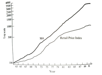
First, in the 'gold standard' system, the supply of money in the economy was determined automatically by the combination of abroad inflows and many banks' behavior. The government had s direct role in this story, even after the note issue was centralized. Second, it was obvious to all observers that periods of inflation followed periods of gold inflows, i.e., rises in the money supply-hence, the formulation of the Quantity Theory of Money. In its simplest form, the aggregate price index will be proportional to the money stock. This should not be objectionable since a 'price' is the number of units of money that exchange for a unit of a good. If there is twice as much money for the same volume of goods, you would expect average prices to double. Figure 3.3 shows index numbers for the broad money stock M4 and the retail price index (RPI). While there may have been some relationship between these two series in the past, the dramatic growth I M4 relative to prices in the 1980s has raised doubts about the monetarist strategy and led to the abandonment of monetary targeting. This does not mean that there is no connection between money and inflation, only that innovations in the financial system have made these connections harder to identify (see Chapter 8).

In the Classical system, causation ran from money to aggregate prices, but money was not in the control of the government. Relative prices adjusted in individual markets to equate demand and supply, so there was no role for the government in general.

If There Is No Role of the Local Government in Adjusting Relative Prices, Does It Affect the World's Budget?

The answer to this is very simple. Budgets were an exercise in raising revenue to pay for government expenditures. The guiding principle was the balanced budget' so that taxes were set to raise just enough money to pay for the government's intended expenditures. Something changed. What was it? There were, in fact, two major changes one was structural, and the other was intellectual.

Figure 3.3 Money stock and the price level (1963 = 100). Source: DataStream.

The important structural change was the break from gold. This happened piecemeal but was completed by the time the post-Second World War domestic and international monetary system was established. In place of gold in the banking system's reserves were the liabilities of the Treasury and the Bank of England. The fact could not be avoided that monetary policy was now a central policy concern. For twenty years or so, however, monetary policy seemed to take a back seat to fiscal policy.

As we have seen, fiscal policy was the product of the Keynesian revolution in economic thought. Monetary policy in the two decades after World War Two was largely passive. This arose from the commitment to fix the exchange rate. The connection may not seem obvious, but it is very important. If too much money were circulating in Britain, people would want to spend more abroad on goods or investments. To spend abroad, domestic residents had to buy foreign exchange. The Bank of England had to buy the extra pounds offered with dollars to stop the price of foreign exchange from rising.

In other words, if too much money was generated, the bank had to buy it back with foreign exchange reserves. Hence, even if too much money were 'printed,' this would lead to a loss of reserves and a subsequent policy reversal long before it has caused inflation of prices. In a sense, fixing the exchange rate is a rule controlling the money supply and, in effect, ties domestic inflation to the world economy.

The only monetary problem that governments had was how to finance the budget deficits that fiscal policy required without leading directly to a loss of reserves. The problem arises from the fact that short-term government debt is a reserve asset for the banking system. So government borrowing from banks can lead directly to banks increasing the money supply. This is what is normally meant by the government 'printing" money. Inconsistencies in this policy area were met in the 1960s by the imposition of quantitative ceilings on bank lending, which, in effect, swept the problem under the carpet by inhibiting the major clearing banks and stimulating the growth of uncontrolled 'secondary' banks.

Two separate areas of academic work laid the groundwork for early monetarism; Milton Friedman contributed to both. The first was the demonstration that the aggregate demand for money in the economy was a stable function of a few variables. This underlay the analysis offered on the effects of increasing the money supply. The rule of thumb was that a rise in the money stock would have a transitory effect on output after about a year and a permanent (upward) effect on prices after about two years. Other important ideas were developed in the context of the famous Phillips Curve (see Chapter 7). This had become widely accepted in the early 1960s as it established a stable trade-off between inflation and unemployment. If the government was prepared to accept an increase in inflation, it could achieve a reduction in unemployment. The revised theory, however, held that if unemployment were reduced below what Friedman called the 'natural' rate, this would not lead to stable inflation but ever-accelerating inflation.

The combined effect of these two developments was to reassert the validity of the Quantity Theory, at least in the long run. Expanding the money stock could stimulate employment and output temporarily. Still, ultimately this effect would be reversed (or even more than reversed), and the only lasting effect would be a rise in prices in proportion to the rise in the money stock. However, the relevance of these ideas was not generally appreciated in the United Kingdom in the late 1960s when they hit the academic community because, as we have seen, the money supply was effectively controlled by the commitment to pegging the exchange rate as well as by direct controls on the banks. Indeed, it is ironic to recall that after the election of 1970, an incoming Tory government inherited a balance of payments surplus, a budget surplus, and a controlled money supply. The next three years changed all that in a way that was a little short of disastrous.

Again, a structural change was integral to what followed. There were two important changes in 1971. The first was the floating of the dollar, which was implied by the Nixon speech of 15 August. The second was the domestic reform known as Competition and Credit Control, introduced in September. This removed the direct controls on the banking system and had the effect of allowing the money supply, as measured by M3, to grow at a rate in the order of 25 percent per annum until the end of 1973 (see Figure 3.1, this shows M4 growth which is now the standard broad money series; M3 growth was faster than that of M4 in the 1971-73 period). It should be no surprise that inflation reached about 25 percent in 1975 (the highest level of peacetime inflation in the United Kingdom since the sixteenth century). The reason that this was now possible was that the pound was floating.

Why Did Floating The Pound Have Anything To Do With Competition And Credit Control?

Monetary expansion with fixed exchange rates did not lead to inflation because, as we have seen, the Bank of England would buy back pounds with dollars to stop the exchange rate from falling. Another way to think of this is that tying the value of our money to that of the dollar also ties our inflation rates together within limits. Monetary expansion with floating rates, however, is very different. Since the central bank does not buy back the pounds, people with too many pounds spend them. If the economy is spending more than its income, there is a balance of payments deficit. The value of the pound vis-à-vis the dollar starts to fall. This leads directly to the sterling price of imports rising, and prices in the shops soon follow. Under fixed exchange rates, a monetary expansion leads directly to a reserve outflow. With floating exchange rates, it leads to a depreciating currency and a build-up of domestic inflation as price rises feed through in wage rises and so on.

The expansionary monetary policy of 1971-73 was accompanied by a major fiscal stimulus following the March 1972 Budget of Mr. Barber, which set the course for the massive budget deficits of the late 1970s. There can be no serious doubts that the policies of the 1971-73 period were irresponsible or incompetent (or both), and Britain suffered from them for at least the next decade. The central Monetarist proposition is substantially borne out by the evidence of this period, as Figure 3.1 (see also Figure 1.2) demonstrates. A massive monetary expansion led to a short-lived boom and, later, rapid inflation. This would have been true with or without the Oil Crisis, which just worsened things. (One of the great myths that survived this time is that the oil shock caused British inflation. West Germany had the same oil shock but did not have inflation above 8 percent. Britain's inflation was undoubtedly dominantly homegrown.)

Another irony of the 1970s experience is that the Labour Government of 1974-79 was the first to admit that the Monetarists were right. The Labour Chancellor of the Exchequer, Denis Healey, introduced cash limits on Government expenditure and money supply targets. In this sense, everybody became a Monetarist for a while. Without fixed exchange rates or the gold standard, there has to be some method for controlling the money supply to avoid runaway inflation. There is still disagreement, even within the Monetarist camp, about how rigid monetary control needs to be. More importantly, perhaps, there is disagreement about how fast ongoing inflation can be brought down by monetary control. Many, including Friedman himself, have argued for gradualism because the very tight policy has real severe effects before it works to control prices. Others like Hayek favor a 'short, sharp shock.'

Monetary policy targets were central to the policy strategy of the Thatcher Government after 1979. A gradual tightening of monetary growth rates was intended to bring down inflation over time. However, the Thatcher Government did not stick to its monetarist strategy for very long. There is continuing controversy as to what extent monetary policy was genuinely the cause of the 1980 recession (see Chapter 12 and Chrystal, 1984). However, in practice, monetary targeting was abandoned by the Thatcher Government in the early 1980s, and partly due to this, inflationary forces were allowed to build up again. (For an extended discussion of the financial innovation of the 1980s and monetary policy problems in the late 1980s, see Chapter 8.) Broad money growth of 15-20 percent per annum was permitted for several years in the mid-1990 (see Figure 3.1). Eventually, money supply targets were replaced by exchange rate targets. However, the exchange rate target had to be abandoned in September 1992 due to speculative pressure.

The reasons for the abandonment of monetary targeting were that the favored measures of money - originally M3 and later M4- ceased to have the same stable relationship with the economy as had existed in 1970 (apparently). Hence, discretion dominated rules in monetary affairs. Unfortunately, judgment has to be good for policy to be good. Such was not the case in the late 1980s.

In 1993 the United Kingdom found itself again in search of a guiding principle for monetary policy, having suffered over 550 percent cumulative inflation in two decades but seemingly having learned very little from experience. Chancellor of the Exchequer, Norman Lamont, adopted guiding ranges of MO and M4 as potential monetary policy indicators. Even though M4 had been abandoned earlier as an indicator because of the instability of its link with the economy (velocity). Meanwhile, the United Kingdom had lurched from the excessive looseness in the monetary policy of 1988 to the excessive tightness of 1990-92. The Monetarist concern that discretionary monetary policy would add to economic cycles rather than smooth them was substantially supported by the UK experience. This is particularly alarming given that the government which delivered these extreme lurches in policy was meant to be sympathetic to monetarism.

Thatcher and Monetarism

The monetarism outlined above can be associated with statements such as, 'There is a stable demand function for money' or 'Inflation is always and everywhere a monetary phenomenon.' It is possible to agree with these and yet disagree with the policies pursued by Prime Minister Margaret Thatcher in 1979-91, though she was commonly labeled 'Monetarist.' Indeed, many true Monetarists doubt that Mrs. Thatcher was a Monetarist. Her government largely ignored its monetary targets even when it had them, abandoned monetary targeting, and rekindled in. Action, and then opted for a very costly exchange rate target. As monetarism aims to achieve a stable monetary environment without recourse to big swings in policy stance, the Thatcher incumbency would score very low in Monetarist popularity polls. The guiding principles of Thatcherism were, in fact, much more closely related to nineteenth-century liberal laisser-faire economics. It is based on a belief in the benefits of the outcome of the working of free market forces, with government participation reduced to a minimum. It is true that many Monetarists, including Milton Friedman, would support the liberal agenda. This is, perhaps, the reason for the confusion of terminology. However, this is the Friedman of Capitalism and Freedom and Free to Choose, rather than the Friedman of Monetary History of the United States and Monetary Trends in the US and UK.

Thatcherism, then, is associated with a particular view about the role of government in the economy. It is the minimalist view of the 'get Big Government off the back of the People' approach, and the "Taxation is theft" view. Questions about the appropriate role of government in a market economy and about monetary institutions and their control are quite separate. The underlying relevance theory to the former is not traditionally regarded as part of macroeconomics. Accordingly, a full discussion goes beyond the scope of this book. Alt and Chrystal (1983) offer an introduction to the main issues.