Fall 2022 Multiple Linear Regression – Biostatistics Mid-term Exam Solution: The University of California

Here are the questions and solutions for a fall 2022 mid-term exam on biostatistics. The test assesses students’ knowledge of using SAS to perform multiple linear regression. Feel free to use the practice questions and answers for your revision and exam preparation. Remember, we are at the service of students looking to pay a professional to take a biostatistics exam for them. We have assembled a competent team of experts knowledgeable on the critical topics of this subject. Submit your exam details to us and we’ll connect you to a skillful multiple linear regression exam helper. Our website is the ultimate destination for students who want to score the best grades on their biostatistics exams.

Question 1: (Use SAS to get the outputs)

The pressure data description

Data from 20 patients contain the blood pressure information. Our Interest is to see if a relationship exists between blood pressure and other variables age (in years), weight (in kgs.), body surface area (BSA), pulse, Body Mass Index (BMI), and height (m.). If there is any relationship, how these variables can affect the blood pressure (BP).

Get the data pressure in the permanent library HW4 (First create HW4 permanent library in your computer, then import)

libname HW4 'C:\Users\LamicHR\Desktop\EVMS\Teaching\2019\Fall 2019\Biostatistics II\Week 4 Multiple Linear Regression Part I ';
data pressure;
set hw4.pressure;
run;

What are the dependent and independent variables?
Dependent variable – blood pressure (BP)
Independent variables – age, weight, body surface area (BSA), pulse, height, BMI
Calculate the multiple correlations and construct the scatter plots to see the collinearity between these variable

proc corr data=pressure;
var bp age weight BSA pulse height BMI;
run;

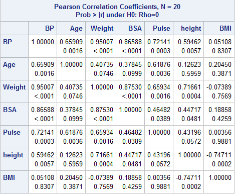
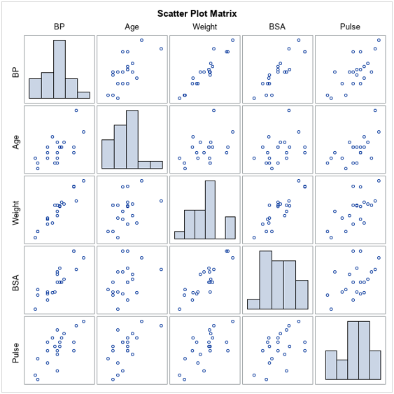
From the results in part (b), do you suspect multi-collinearity of the data? Explain with reason/s.

Yes, there is multi-collinearity in the data. This is because a strong linear relationship exists between some pairs of the independent variables.

- Weight and BSA are highly correlated with a correlation coefficient of 0.8753.

- Weight and Height are highly correlated with a correlation coefficient of 0.71661.

- BMI and Height are highly correlated with a correlation coefficient of -0.74711.

Write down the equation of multiple linear regression of BP on Age, Weight, BSA, Pulse, Height, and BMI.

proc reg data=pressure;
model bp=age weight BSA pulse height BMI;
run;

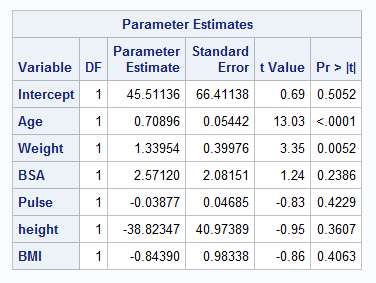
BP = 45.51136 + 0.70896*Age + 1.133954*Weight + 2.5712*BSA – 0.03877*Pulse – 38.82347*height – 0.8439*BMI

Fit the multiple linear regression of BP on Age, Weight, BSA, Pulse, Height, and BMI by using SAS. Don’t forget to calculate Variance Inflation Factor.

proc reg data=pressure;
model bp=age weight BSA pulse height BMI/VIF;
run;

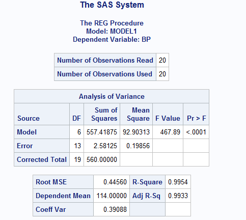
What is the R2 value? Do you think this model is an excellent model to fit the data? Explain why this R2 is too high?

R2 = 0.9954.

The model might not be excellent to fit the data, because of the suspiciously high coefficient of determinant (R2).

This R2 is too high because there is an overfitting of the regression model, that is, the model is describing the random error in the data instead of describing the relationship between the variables.

Check the Variance Inflation Factor? Do you suspect multi-collinearity in this model? Explain with reasons.

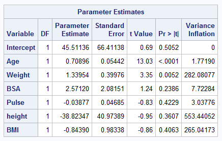
Yes, there is multicollinearity in the data. This is because of the high VIF values for some of the predictor variables; a VIF value of > 10 suggests multicollinearity. In our case multicollinearity arises because of Weight, Height and BMI.

Remove the variable with highest unusual VIF and re-fit the model again and check the VIF. Do this until you find all VIFs are in acceptable range, the final model is the full model you want. What variables are there in the full model?

Age, BSA (body surface area) and Pulse

proc reg data=pressure;
model bp=age BSA pulse/VIF;
run;

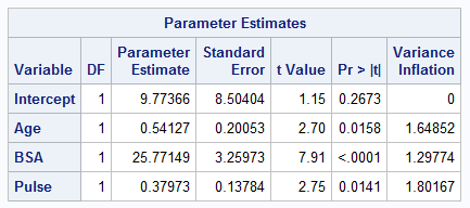
In the full model from part (h), are all the independent variables significant predictors of BP? Explain.

Yes, all the independent variables in the full model are significant predictors of BP. This is because they all have a p value of less than 0.05 (significance level).

If there are any non-significant predictors in the full model, remove them and re-fit the model with significant predictors only. This is called the reduced model. What variables are there in your reduced model?

This is not applicable since all the independent variables in our full model are significant predictors of BP.

Question 2: The reduced model contains Age and Weight as the significant predictors. Fit a multiple regression model of BP on Age and weight

proc reg data=pressure;
model bp=age weight/VIF dwprob;
run;

Write down the regression equation of this model.

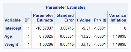
BP = -16.57937 + 0.70825*Age + 1.03296*Weight

Are all assumptions, LINEC, satisfied? Explain in details.

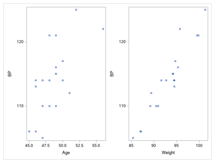
Linearity is satisfied – there is a linear relationship between the dependent variable and the predictors.

proc sgscatter data=pressure;
plot bp*age bp*weight ;
run;

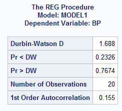
Independence of error terms – This assumption is met. The Durbin-Watson D value (1.688) is between 1.5 and 2.5, which confirms the absence of first-order autocorrelation.

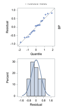
Normality – This condition is satisfied. The Q-Q plot and histogram of the residual from the Fit Diagnostics show that the residuals are normally distributed.

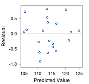
Errors have a constant variance – this assumption is satisfied. This plot of Residuals by Predicted values from the Fit Diagnostics shows this.

Collinearity – The assumption of little or no multicollinearity is satisfied. There is no multicollinearity among the independent variables. All VIF values are <= 10.

Interpret all parameter estimates of the reduced model?

The intercept is -16.57937. This is the measure of Blood pressure when all the other variables are held constant.

The coefficient of Age is 0.70825. This means that when all the other variables are held constant, a unit increase in Age increases Blood pressure by 0.70825.

The coefficient of Weight is 1.03296. This means that when all the other variables are held constant, a unit increase in Weight increases Blood pressure by 1.03296.

Interpret the R2 of this model.

R2 of 0.9914 means that 99.14% of the variation in Blood pressure is explained by Age and Weight.

Write down the fitted (predicted) equation of this model.

Y ̂=-16.57937+0.70825(Age)+1.03296(Weight)

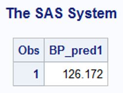
What could be the predicted blood pressure of a person who is 63 years old and has weight 95 kg.?

data predicted;
set estimates;
BP_pred1=intercept+63*age+95*weight;
BP_pred2=intercept+90*age+35*weight;
run;
proc print data=predicted;
var BP_pred1;
run;

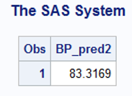
What could be the predicted blood pressure of a person who is 90 years old and has height of 35 kg?

proc print data=predicted;
var BP_pred2;
run;