Studying 101: Questions to Help You Study for and Succeed in Your End-Term Exams Specifically on Predicting Other Firm’s Actions
We offer the best studying tips to students in the blog below. This blog will introduce you to questions you will likely encounter on your microeconomics end-term exams, and also show you how to answer them. The blog focuses on questions on the topic called predicting other firms’ actions. You will mainly find questions on duopoly, oligopoly, and game theory. Find out the best way to study and succeed in your exams in the content below.
Explain and illustrate the concepts of oligopoly using Cournot’s, Edgeworth’s, and Hotelling’s spatial models
- Cournot
Duopoly is a situation where two firms are competing for a particular market. The most famous duopoly theory is also one of the first, that produced in 1838 by Augustin Cournot, a pioneer French economist. His contribution lay in showing that if a firm could make a particular assumption about its rival, we could have a theory of duopoly just as we had theories of competition and monopoly. The crucial assumption a firm had to make was to assume that the other firm would not change its output. This enabled each firm to decide how to deal with 'the rest of the market' not served by the other firm.
In order to simplify the problem Cournot assumed that the firms owned identical mineral-water springs, side by side, and thus had AC = MC= 0. Thus, only revenue would be affected by output and sales. They were assumed to know what the total demand curve for mineral- water was. Figure 8. 1 is an illustration of Cournot's duopoly model. The line DQ is the AR (demand) curve, and DQ1 is the MR curve, (OQ1=Q1Q) OQ is the AC=MC curve. Thus, with only one firm, the profit-maximizing output would be Q, where MC (=0) is equal to MR (=0). Thus, the monopolist would produce 50% (Q1) of the potential sales (Q).
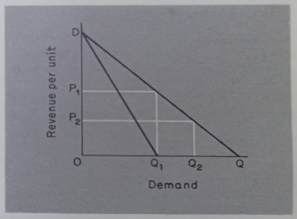
Fig. 8.1 Cournot's duopoly model
We can now see how the firms interact. In the dynamic process
A sees B is not producing and produces Q, the monopoly output, and sells it at price P1 (50% of Q)
B sees A producing Q, (50% of Q) and produces QQ, (50% of Q1Q) and sells it at price P2 (25% of Q)
A sees B producing 25% of Q and produces 50% of (Q-B's (37.5% of Q output) and sells it at price between P1 and P2 (37.5% of Q)
B replies by producing [100-37.5/2] % of Q (31.25% of Q)
Convince yourself that this process will proceed until each duopolist produces 33.3% of Q (in which case 50% of (100-33.3) % of Q is also 33.3%) and sells at 33.3% of OD.
Thus, each firm has a reaction function to produce [100-rival's %/2] Q. If we extend the process to three firms, we find output settles at 25% Q per firm, and we can generalize the result to more firms, with each producing (1/n+1) Q. when there are n firms.
This was very satisfying to classical economists who thus saw a smooth transition between monopoly with an output of ½Q and a price of ½ D and competition with an output of and a price of (1/ n+1) Q and a price of (1/n+1) D for each firm.
- Bertrand and Edgeworth
The simplicity and attractiveness of Cournot's results did not preserve them from criticism. Bertrand suggested that the crucial assumption was suspect.
Why should firms assume others would keep the output constant when in fact they did change Perhaps assuming rivals’ prices to be would be more plausible.
Edgeworth (1881) took these ideas further and showed that a model where each firm rivals' price constant did not produce a solution. A crucial additional assumption is neither duopolist can supply the "whole" (Q), his limit is G (firm A) and g (firm B), as shown in Figure 8.2.
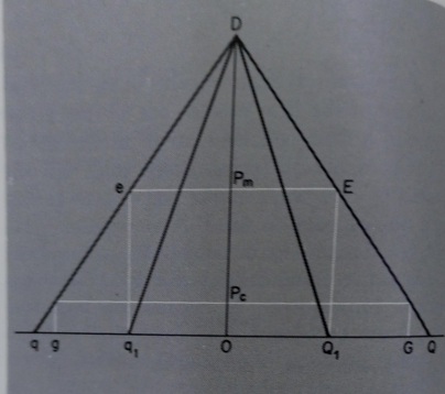
Fig. 8.2 Edgeworth’s duopoly model
We can again follow through the stages of a dynamic interaction:
A sees B is not producing, and produces Q1 the monopoly output, and sells it at the monopoly price Pm
B sees A Producing Q1 at price P and undercuts, his price slightly, taking away all his customers
A retaliates
The process continues until one firm reaches the output limit G or g. The other firm can then raise the price, for instance back up to P... and restart the process.
Thus, Edgeworth's model is both unstable and indeterminate and thus cannot predict price and output for the duopolists. Much later Stackelberg (1932) showed that stability could only be found in unusual conditions. Firms could be expected to learn to anticipate rival's actions and such firms were termed "leaders' by Stackelberg. Those who merely reacted to others were called 'followers". He showed that it was necessary to have at least one 'follower in a market for it to be stable.
So, we can expect to find oligopolies characterized by bouts of price-cutting which may drive prices below long-run marginal cost, as we saw in Chapters 5 and 6. The ways in which firms have actually coped with this problem and the resulting pricing methods are detailed in the further reading by Scherer.
- Hotelling
In 1929 Hotelling produced one of the most interesting models of spatial competition or competitive location. Its interest lies in its two main conclusions: first that duopoly can be stable when firms are not completely free, for instance when they cannot move, and second that under competition firms have the incentive to locate in the center of a market. Figure 8.3 shows the simplest model where location is only possible at points along a line a - b.
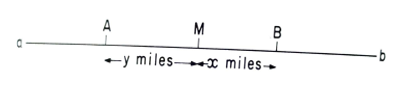
Fig. 8.3 Hotelling's spatial duopoly model
There are two firms located at A and B respectively. The customers are equally spaced along the line ab. Transport cost is c per ton-mile and so the transport cost to a customer at M is cy for good A and ex for good B. If customer M is indifferent (on price) between A and B this is because of the distance and production price. Thus, price cuts will extend the market for a firm, but so long as a firm can compete at all M (the indifferent customer) will be nearer and nearer to the less competitive firm. A customer at a will be the last customer retained by A, and a customer at b, and the last one retained by B. Thus, firm A can attack firm B either by cutting price or by moving towards B's "protected' market.
Explain the notion of oligopoly using the kinked demand curve.
Sweezy's model relies on the fact that in an oligopoly (or duopoly) situation what each firm does will affect the others. Thus, if one cuts the price it will tend to draw customers from the others, and so they will feel compelled to retaliate. However, a price rise will probably not be followed, particularly if the rival firms are concerned to increase their market share. If we translate these assumptions into a demand curve, we find that it has a 'kink' at the current price, as in Figure 8.5. The marginal revenue for the upper AR curve does not continue with the MR for the lower AR curve. Assuming that MC= MR at the current price, costs change considerably, say from MCa to MCh altering the profit-maximizing price. This provides the theoretical explanation for oligopoly being unwilling to change prices. We could go on to suggest that they would then attempt non-pr competition, such as advertising and 'special offer which have no direct price-equivalent. This describes quite well the behavior in some oligopoly markets such as the sale (in the UK) of petni detergents, cigarettes, and beer. Thus, we have a theory that explains observed behavior, with the marginalist framework.
This then is the great achievement of Sweezy’s approach: it retains oligopoly within the marginal analysis, with the individual firm having a dem curve that sums up rivals' reactions in the same way as a price-makers does.
However, the great achievement has been, a fact, to be able to disregard many of the choices open to competitors. We still do not have an analysis that takes into account all of the possible actions of competitors. So far, the theories have limited the possibilities open to all the firms.
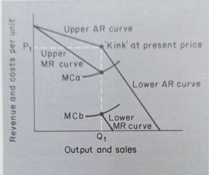
Fig 8.5 The kinked oligopoly demand curve
Definition of Terminologies used in Game Theory
Skill is an element in conventional games; in game theory, all players are assumed to be skilled (equally). This is a simplification that can be removed if necessary.
Chance is similarly removed from our simple version of Game Theory by assuming that we can forecast future events with certainty.
Players Each participant is termed a player. It is often the process of trying to determine how many players are actually involved which provides valuable insights into a situation. We might start off in a wage negotiation by assuming unions and employers' organizations were involved, but we might realize that neither side was a monolithic bloc. The unions might have different interests, as might different employers, and within unions, the shop stewards might differ from the leadership and the workers themselves. The government and even the customers might become players in certain circumstances. The same is true of oligopolies where the customers, government, and potential entrants to the industry are all possible players.
Strategy Players choose which strategy to play. Although we use simple examples such as reducing the price or holding it at a given level, strategies always involve a number of individual moves. Price-cutting, for instance, involves all that is necessary to take advantage of the cut, such as advertising. and increased production.
Payoffs are what results when A plays one strategy and B plays another. In Figure 8.6 the payoffs to A in terms of market-share are shown in top-right- hand corner of the boxes.
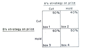
Fig 8.8 Game Theory: pay-offs
Preferences exist between the payoffs. These are a result of the firm's objectives. For instance, a market share maximizer would prefer box 3 to box 1, but would only be able to decide between boxes 1 and 4 (which both offer 50% of the market) by referring to another objective such as profit. An important characteristic of preferences is that they are ordinal i.e., they cannot be added together so there is no way of adding up the preferences of different players to calculate what is best for all of them One of the great achievements of game theory is the ability to reveal situations in which no firm will have the incentive to change, the 'stability' which duopoly sought.
Decision criteria are needed to choose between strategies because each strategy has a number of different preferences associated with it. Presumably, there is no way of knowing the probability of each occurring, so the decision criterion must cat for the possibility of anyone resulting from the choice of strategy.
One possibility is for the firm to be pessimistic, assume that the worst could happen, and evaluate each strategy from this point of view. This would lead them to choose the strategy for which t worst outcome (called the minimum of t strategy, was better than the minima of the other strategies. Choosing the strategy with the high minimum is called using the maximin decision criterion. Likewise, a gambler might assume that the best would happen and so would choose the strategy with the highest maximum (the strategy with the best outcome), and this is called the maximax decision criterion.
If we note the preferences which we discussed in Table 8.6 we obtain Figure 8.7. If A assumes the worst (uses the maximin criterion) he will choose to car price. This is because the minimum of this strategy is his third preference whilst the minimum holding price is the fourth preference. In this particular case, the maximax criterion gives the same choice of strategy, as the cutting price has the highest maximum (the first preference). In a situation like this, where almost any decision criterion (and there are others) would choose one strategy it is said to dominate the other(s). A more common situation is where one strategy will never be chosen because there will always be another that it is better, and this strategy is said to be dominant.
Competitive is a term that is used in a very restricted sense in game theory. We call a game competitive to distinguish it from a situation where the players intend to be cooperative. However, there is a further dimension, the payoffs. If what one player gains is lost by the others (e.g., market share) then the game is constant-sum. However, most economic situations are not constant-sum, because they either involve profit, which varies with price, or, more generally, because the players can impose costs, or confer benefits on non-players. This is unfortunate because some of the most powerful theorems of game theory apply to constant-sum games. (They are often referred to as zero-sum games, but simple constant games, such as market share, can be espremed zero-sum if the need to be, e.g. market shares be expressed as 45% +55%-100% or as +5%0.) However, many of the insights do game theory are still applicable to non-const sum games.
Illustrate the prisoner’s dilemma using game theory
Insights from games: the prisoner's dilemma Here the basic assumption is that two prisoners have committed a crime together but that the police are not sure that they have enough evidence to secure a conviction in court. The police hold the separately to prevent communication between them and offer each of them lighter sentences if they confess to the crime. The usual sentence is ten years, but helping the police by confessing would reduce this to two if it secured the conviction of the other criminal. If, however, they both confess they know that this will only reduce their sentence marginally, say to eight years. We can represent the payoffs to them in Figure 8.9. We have, of course, assumed that if neither confesses there will not be enough evidence to convict them. What should each prisoner do? If they use the maximin criterion they will choose the strategy with the highest minimum. Remaining silent could mean going to prison for ten years whereas the worst result of confessing is eight years. So, each would choose to confess, useful for the police but disastrous for the criminals.
This game contains the essence of many oligopoly problems. Firms could cooperate and achieve higher prices and profits but are forced to compete on price through their distrust of their rivals. What are the crucial factors?
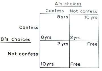
Fig 8.9 Game theory: the prisoner’s dilemma
The first is communication. If the prisoners had been allowed to communicate, they would have been able to agree on the best solution (for them) of not confessing. This obviously has its parallel in oligopolies where agreements (communication) are used to prevent price competition. (For more subtle forms of communication see the further reading by Scherer.) Thus, governments who wish to encourage price cutting by oligopolists make agreements between firms illegal.
The second important factor is the possibility of achieving the prisoners' aim by their having some reason for never confessing. This could be for a variety of reasons, but the net result is that the strategy of confessing is externally dominated, i.e., not chosen. Again, the government can externally dominate some of the oligopolists' strategies, such as preventing price increases by having some form of price control.